using Pumas
using PumasUtilities
using Random
using CairoMakie
using AlgebraOfGraphics
using DataFramesMeta
using CSV
PK02 - One-compartment oral dosing
1 Learning Outcome
By the application of the present model, we will learn how to model orally-administered drug data with a first order input model with and without a lag-time.
2 Objectives
In this exercise, you will learn how to:
- Simulate an Oral One Compartment (with/without lag-time) model (assuming oral bioavailability of 100%). Remember, since this is an oral medication, the interpretation of V includes bioavailability (i.e., it is really estimating V/F).
- Write a differential equation for a one-compartment model.
3 Background
Before constructing a model, it is important to establish the process the model will be following and a scenario for the simulation.
Below is the scenario for this tutorial:
- Structural model - 1 compartment with first order absorption (without/with Lag time)
- Route of administration - Oral
- Dosage Regimen - 100 μg Oral
- Number of Subjects - 1
This diagram describes how such an administered dose will be handled, which facilitates building the model. 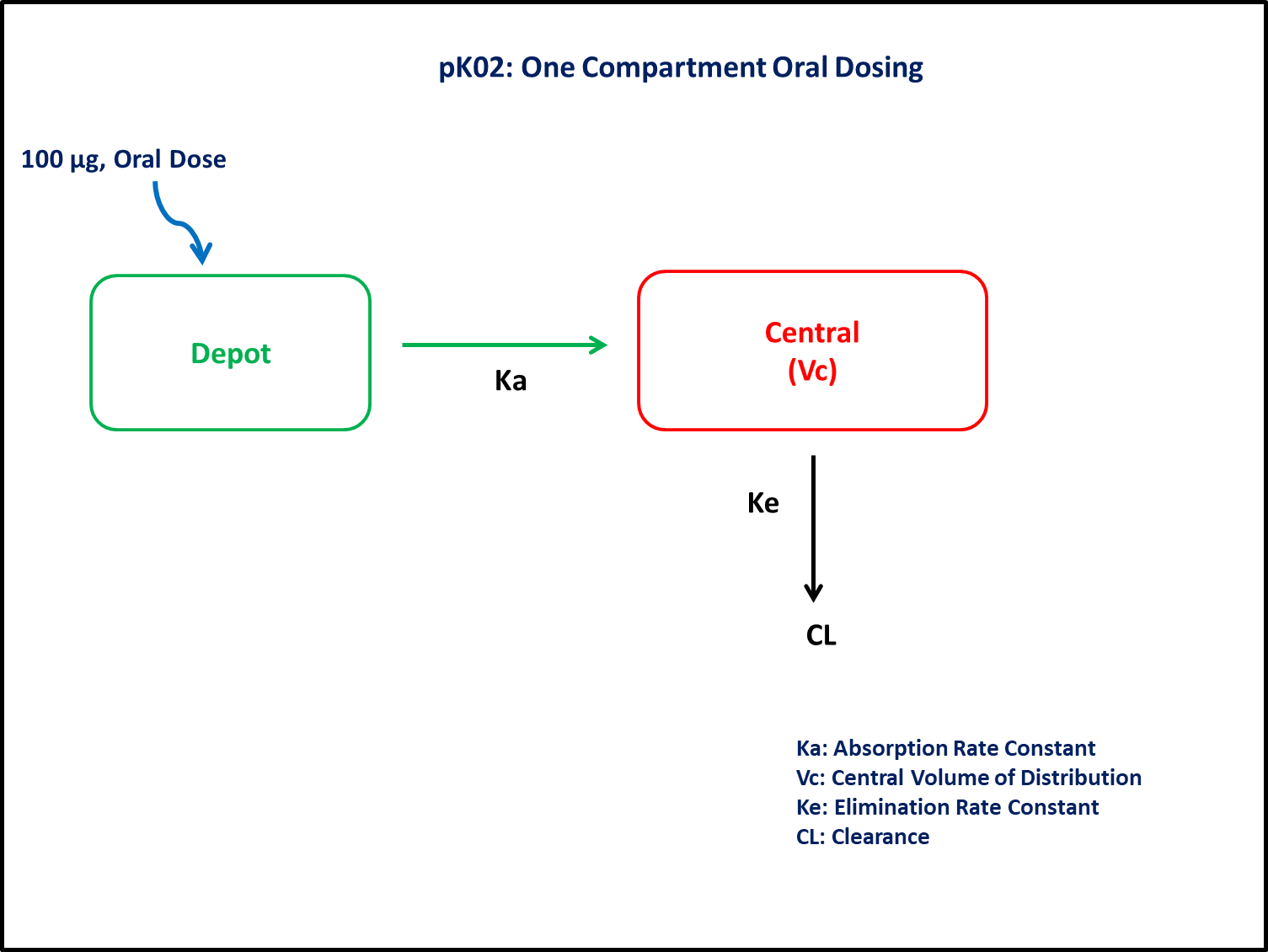
4 Libraries
Call the required libraries to get started.
5 Model
In this one compartment model, we administer the dose in Depot compartment at time = 0.
Addition to Model Blocks
Take note that this model includes a lag time in the @param and @dosecontrol blocks.
pk_02 = @model begin
    @metadata begin
        desc = "One Compartment Model with lag time"
        timeu = u"minute"
    end

    @param begin
        """
        Absorption rate constant (1/min)
        """
        tvka ∈ RealDomain(; lower = 0)
        """
        Elimination rate constant (1/min)
        """
        tvkel ∈ RealDomain(; lower = 0)
        """
        Volume (L)
        """
        tvvc ∈ RealDomain(; lower = 0)
        """
        Lag Time (mins)
        """
        tvlag ∈ RealDomain(; lower = 0)
        Ω ∈ PDiagDomain(3)
        """
        Proportional RUV
        """
        σ²_prop ∈ RealDomain(; lower = 0)
    end

    @random begin
        η ~ MvNormal(Ω)
    end

    @pre begin
        Ka = tvka * exp(η[1])
        Kel = tvkel * exp(η[2])
        Vc = tvvc * exp(η[3])
    end

    @dosecontrol begin
        lags = (Depot = tvlag,)
    end

    @dynamics begin
        Depot' = -Ka * Depot
        Central' = Ka * Depot - Kel * Central
    end

    @derived begin
        """
        Concentration (μg/L)
        """
        cp = @. Central / Vc
        """
        Concentration (μg/L)
        """
        dv ~ @. Normal(cp, sqrt(cp^2 * σ²_prop))
    end
end
PumasModel
Parameters: tvka, tvkel, tvvc, tvlag, Ω, σ²_prop
Random effects: η
Covariates:
Dynamical system variables: Depot, Central
Dynamical system type: Matrix exponential
Derived: cp, dv
Observed: cp, dv
Take note of the derived block!
- Do not forget the
@.. - Be sure to code for the correct Residual Unexplained Variability (RUV) in the derived block. This is an example of a model with proportional RUV.
6 Parameters
The compound follows a one compartment model, in which the various parameters are as mentioned below:
Ka- Absorption Rate Constant (min⁻¹)Kel- Elimination Rate Constant (min⁻¹)Vc- Central Volume of distribution (L)tlag- Lag-time (min)Ω- Between Subject Variabilityσ- Residual error
These are the initial estimates we will be using in this model exercise. tv represents the typical value for parameters.
The first set of estimates does not include lag time and has the typical values for absorption rate constant tvka and elimination rate constant tvkel as the same values.
The second set of estimates includes a lag time estimate and has different values for tvka and tvkel.
param = [
    (
        tvka = 0.013,
        tvkel = 0.013,
        tvvc = 32,
        tvlag = 0,
        Ω = Diagonal([0.01, 0.01, 0.01]),
        σ²_prop = 0.015,
    ),
    (
        tvka = 0.043,
        tvkel = 0.0088,
        tvvc = 32,
        tvlag = 16,
        Ω = Diagonal([0.01, 0.01, 0.01]),
        σ²_prop = 0.015,
    ),
]
7 Dosage Regimen
To start the simulation process, the dosing regimen from the background section must be developed first prior to running a simulation.
In this section, the DosageRegimen is mentioned:
- Oral dosing of 100 μg at
time=0
This is how to establish the dosing regimen:
ev1 = DosageRegimen(100; time = 0, cmt = 1)1×10 DataFrame
| Row | time | cmt | amt | evid | ii | addl | rate | duration | ss | route |
|---|---|---|---|---|---|---|---|---|---|---|
| Float64 | Int64 | Float64 | Int8 | Float64 | Int64 | Float64 | Float64 | Int8 | NCA.Route | |
| 1 | 0.0 | 1 | 100.0 | 1 | 0.0 | 0 | 0.0 | 0.0 | 0 | NullRoute |
This is how to create a population of 2 subjects receiving the dosing regimen above. The first subject is simulated with the “No lag”, parameters and the second subject is simulated with the “With Lag” parameters, as they were specified above.
pop = map(i -> Subject(id = i, events = ev1), ["1: No Lag", "2: With Lag"])Population
Subjects: 2
Observations: 8 Simulation
Note
The Random.seed! function is included here for purposes of reproducibility of the simulation in this tutorial. Specification of a seed value would not be required in a Pumas workflow that is estimating model parameters.
Random.seed!(123)Perform the simulation step.
sim = map(zip(pop, param)) do (subj, p)
    return simobs(pk_02, subj, p, obstimes = 0:1:400)
end
Simulated population (Vector{<:Subject})
Simulated subjects: 2
Simulated variables: cp, dv9 Visualize results
From the plot below, we can clearly identify the subject with and without lag time.
@chain DataFrame(sim) begin
    dropmissing(:cp)
    data(_) *
    mapping(:time => "Time (minutes)", :cp => "Concentration (μg/L)"; color = :id => "") *
    visual(Lines; linewidth = 4)
    draw(; figure = (; fontsize = 22))
end
10 Population Simulation
This block updates the parameters of the model to increase intersubject variability in parameters and defines the time points for the predicted concentrations. The results are written to a CSV file.
par = (
    tvka = 0.043,
    tvkel = 0.0088,
    tvvc = 32,
    tvlag = 16,
    Ω = Diagonal([0.04, 0.09, 0.015]),
    σ²_prop = 0.03,
)

ev1 = DosageRegimen(100; time = 0, cmt = 1)
pop = map(i -> Subject(; id = i, events = ev1), 1:100)

Random.seed!(1234)
pop_sim = simobs(
    pk_02,
    pop,
    par,
    obstimes = [0, 10, 15, 20, 30, 40, 60, 90, 120, 180, 210, 240, 300, 360],
)
df_sim = DataFrame(pop_sim)
CSV.write("pk_02.csv", df_sim)
"pk_02.csv"
Saving the Simulation Results
With the CSV.write function, you can input the name of the dataframe (df_sim) and the file name of your choice (pk_02.csv) to save the file to your local directory or repository.
11 Conclusion
This tutorial has demonstrated constructing a one compartment model in Pumas.
We describe the:
- model structure for the process of the drug passing through the system,
- translating processes into ODEs using Pumas, and
- simulating the model in a single patient, with and without an absorption lagtime.