using Pumas
using PumasUtilities
using Random
using CairoMakie
using AlgebraOfGraphics
using DataFramesMeta
PK05 - One-compartment intravenous plasma/urine I
1 Learning Outcome
In this model, both plasma and urine data are collected, which will help to estimate parameters like Clearance, Volume of Distribution and fraction of dose excreted unchanged in urine.
2 Objectives
In this tutorial, you will learn how to:
- Build a one compartment model of a medication that undergoes excretion via urine
- Simulate the model for a single subject and a single dosing regimen, and
- Fit the model to data containing urine sample information
3 Background
Before constructing a model, it is important to establish the process the model will follow and a scenario for the simulation.
Below is the scenario for this tutorial:
- Structural Model - One Compartment Model with urinary excretion
- Route of Administration - Intravenous Bolus
- Dosage Regimen - 250 mg IV Bolus
- Subject - 1
This diagram describes how such an administered dose will be handled, which facilitates building the model. 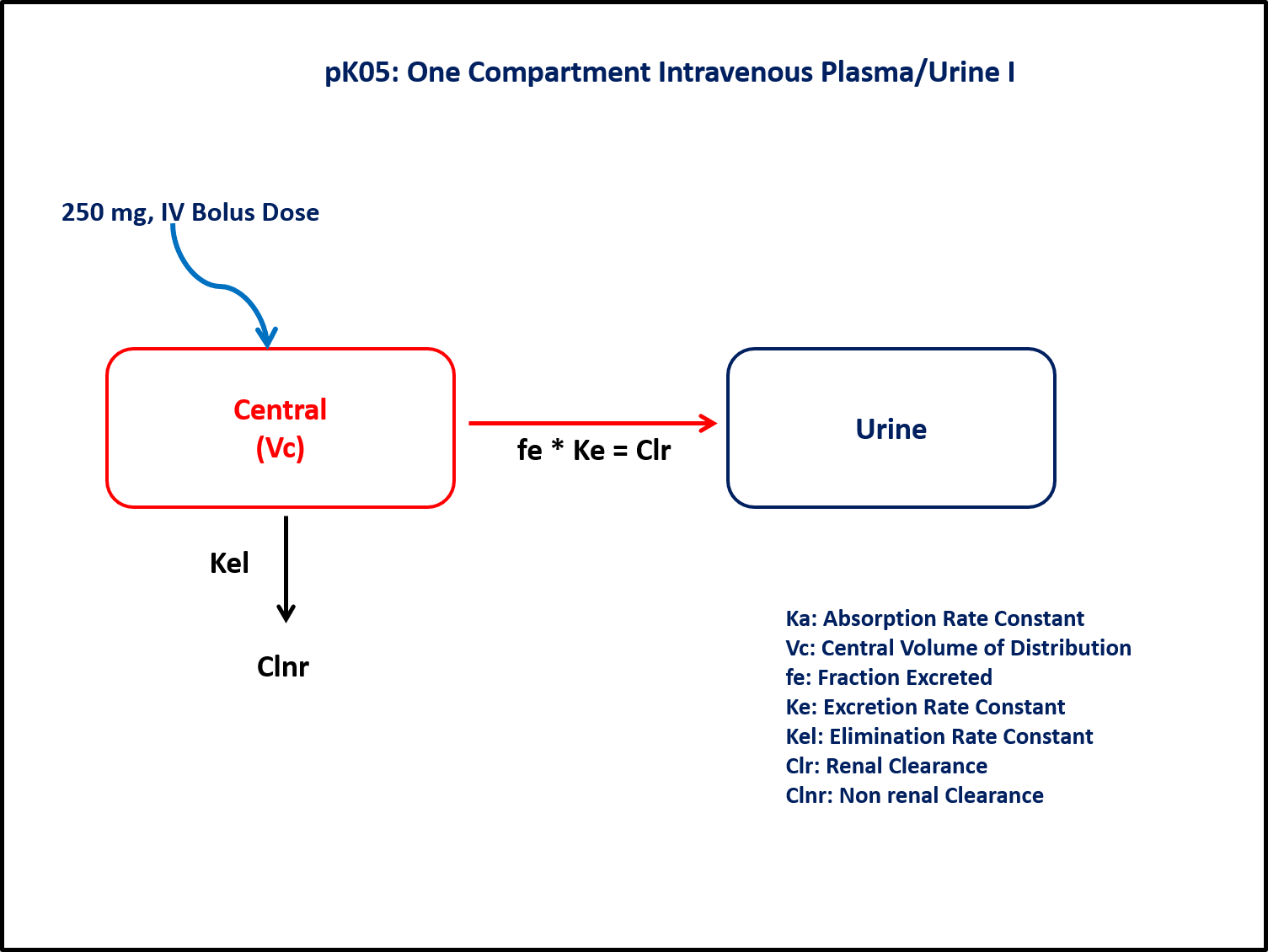
4 Libraries
Call the required libraries to get started.
5 Model
In this one compartment model, we administer an IV dose in the central compartment.
New Urine Compartment in
@dynamics
In the @dynamics block, a Urine Compartment is included. This measures the rate of change in amount over time and calculates the cumulative amount of drug in urine.
pk_05 = @model begin
    @metadata begin
        desc = "One Compartment Model with Urine Compartment"
        timeu = u"hr"
    end

    @param begin
        """
        Volume of Distribution (L)
        """
        tvvc ∈ RealDomain(lower = 0)
        """
        Renal Clearance(L/hr)
        """
        tvClr ∈ RealDomain(lower = 0)
        """
        Non Renal Clearance(L/hr)
        """
        tvClnr ∈ RealDomain(lower = 0)
        Ω ∈ PDiagDomain(3)
        """
        Proportional RUV - Plasma
        """
        σ_prop ∈ RealDomain(lower = 0)
        """
        Additive RUV - Urine
        """
        σ_add ∈ RealDomain(lower = 0)
    end

    @random begin
        η ~ MvNormal(Ω)
    end

    @pre begin
        Clr = tvClr * exp(η[1])
        Clnr = tvClnr * exp(η[2])
        Vc = tvvc * exp(η[3])
    end

    @dynamics begin
        Central' = -(Clnr / Vc) * Central - (Clr / Vc) * Central
        Urine' = (Clr / Vc) * Central
    end

    @derived begin
        """
        PK05 Plasma Concentration (mg/L)"
        """
        cp_plasma = @. Central / Vc
        dv_plasma ~ @. Normal(cp_plasma, abs(cp_plasma) * σ_prop)

        """
        PK05 Urine Amount (mg)
        """
        cp_urine = @. Urine
        dv_urine ~ @. Normal(cp_urine, abs(σ_add))
    end
end
PumasModel
Parameters: tvvc, tvClr, tvClnr, Ω, σ_prop, σ_add
Random effects: η
Covariates:
Dynamical system variables: Central, Urine
Dynamical system type: Matrix exponential
Derived: cp_plasma, dv_plasma, cp_urine, dv_urine
Observed: cp_plasma, dv_plasma, cp_urine, dv_urine6 Parameters
The parameters to define and estimate using the model are as mentioned below:
Clnr- Non renal Clearance (L/hr)Clr- Renal Clearance (L/hr)Vc- Volume of the Central Compartment(L)Ω- Between subject variabilityσ- Residual Error
These are the initial estimates we will be using in this model exercise. Note that tv represents the typical value for parameters.
param = (;
    tvvc = 10.7965,
    tvClr = 0.430905,
    tvClnr = 0.779591,
    Ω = Diagonal([0.01, 0.01, 0.01]),
    σ_prop = 0.1,
    σ_add = 1,
)
7 Dosage Regimen
To start the simulation process, the dosing regimen from the background section must be developed first. From our background, we established the scenario as a single dose of 250 mg given as an Intravenous bolus to a single subject.
The DosageRegimen is specified as:
ev1 = DosageRegimen(250; time = 0, cmt = 1)1×10 DataFrame
| Row | time | cmt | amt | evid | ii | addl | rate | duration | ss | route |
|---|---|---|---|---|---|---|---|---|---|---|
| Float64 | Int64 | Float64 | Int8 | Float64 | Int64 | Float64 | Float64 | Int8 | NCA.Route | |
| 1 | 0.0 | 1 | 250.0 | 1 | 0.0 | 0 | 0.0 | 0.0 | 0 | NullRoute |
This is how to create the single subject undergoing the dosing regimen above.
sub = Subject(; id = 1, events = ev1)Subject
ID: 1
Events: 18 Simulation
Let’s simulate the plasma concentration and the unchanged amount excreted in urine.
Random.seed!()
The Random.seed! function is included here for purposes of reproducibility of the simulation in this tutorial. Specification of a seed value would not be required in a Pumas workflow that is estimating model parameters.
Random.seed!(123)sim_sub1 = simobs(pk_05, sub, param, obstimes = 0:0.1:26)SimulatedObservations
Simulated variables: cp_plasma, dv_plasma, cp_urine, dv_urine
Time: 0.0:0.1:26.09 Visualization
These figures display the drug concentration levels in both plasma and urine samples.
variable_renamer = renamer(
    "cp_plasma" => "Plasma \n concentration (mg/L)",
    "cp_urine" => "Urine \n amount (mg)",
)

plot_df = @chain DataFrame(sim_sub1) begin
    @select :id :time :cp_plasma :cp_urine
    dropmissing([:cp_plasma, :cp_urine])
    stack(Not(:id, :time))
end

plt_rows =
    data(plot_df) *
    mapping(:time => "Time (hours)", :value => "", row = :variable => variable_renamer) *
    visual(Lines; linewidth = 4)

draw(plt_rows; figure = (; fontsize = 22), facet = (; linkyaxes = :none))
By looking at the figure, we can observe that the drug level is decreasing in plasma and increasing in the urine, which resembles normal physiologic function.
When we put the visualization together, we observe the following figure:
plt_join =
    data(plot_df) *
    mapping(
        :time => "Time (hours)",
        :value => "Concentration / Amount",
        color = :variable => variable_renamer => "",
    ) *
    visual(Lines; linewidth = 4)

draw(plt_join; figure = (; fontsize = 22), legend = (; position = :bottom))
10 Population Simulation
This block updates the parameters of the model to increase intersubject variability in parameters and defines timepoints for prediction of concentrations. The results are written to a CSV file.
par = (
    tvvc = 10.7965,
    tvClr = 0.430905,
    tvClnr = 0.779591,
    Ω = Diagonal([0.04, 0.09, 0.0225]),
    σ_prop = 0.0256,
    σ_add = 3.126,
)

ev1 = DosageRegimen(250; time = 0, cmt = 1)
pop = map(i -> Subject(id = i, events = ev1), 1:55)

Random.seed!(1234)
pop_sim = simobs(pk_05, pop, par, obstimes = [0.5, 1, 1.5, 2, 4, 6, 8, 12, 18, 24])
sim_plot(pop_sim)

df_sim = DataFrame(pop_sim)

#CSV.write("pk_05.csv", df_sim)
Saving the Simulation Results
With the CSV.write function, you can input the name of the dataframe (df_sim) and the file name of your choice (pk_05.csv) to save the file to your local directory or repository.
11 Conclusion
Constructing a one compartment model with urine elimination involves:
- understanding the process of how the drug is passed through the system,
- translating processes into ODEs using Pumas,
- explaining the drug elimination process in Pumas, and
- simulating the model in a single patient for evaluation.