using PumasUtilities
using Random
using Pumas
using CairoMakie
using AlgebraOfGraphics
using CSV
using DataFramesMeta
using Dates
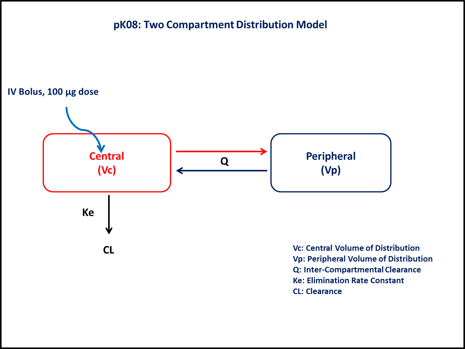
PK08 - Two compartment distribution models
1 Background
- Structural model - Two compartment linear elimination with first order elimination
- Route of administration - IV bolus
- Dosage Regimen - 100 μg IV or 0.1 mg IV
- Number of Subjects - 1
2 Learning Outcome
This exercise demonstrates simulating single IV bolus dose kinetics from a two-compartment model.
3 Objectives
To build a two-compartment model, simulate the model for a single subject given a single IV bolus dose, and subsequently perform a simulation for a population.
4 Libraries
Load the necessary libraries.
5 Model definition
Note the expression of the model parameters with helpful comments. The model is expressed with differential equations. Residual variability is a proportional error model.
pk_08_05 = @model begin
    @metadata begin
        desc = "Two Compartment Model"
        timeu = u"hr"
    end

    @param begin
        """
        Clearance (L/hr)
        """
        tvcl ∈ RealDomain(lower = 0)
        """
        Volume of Distribution (L)
        """
        tvvc ∈ RealDomain(lower = 0)
        """
        Intercompartmental Clearance (L/hr)
        """
        tvq ∈ RealDomain(lower = 0)
        """
        Peripheral Volume of Distribution (L)
        """
        tvvp ∈ RealDomain(lower = 0)
        #Ω ∈ PDiagDomain(4)
        Ω_cl ∈ RealDomain(lower = 0.0001)
        Ω_vc ∈ RealDomain(lower = 0.0001)
        Ω_q ∈ RealDomain(lower = 0.0001)
        Ω_vp ∈ RealDomain(lower = 0.0001)
        """
        Proportional RUV
        """
        σ²_prop ∈ RealDomain(lower = 0)
    end

    @random begin
        η_cl ~ Normal(0, sqrt(Ω_cl))
        η_vc ~ Normal(0, sqrt(Ω_vc))
        η_q ~ Normal(0, sqrt(Ω_q))
        η_vp ~ Normal(0, sqrt(Ω_vp))
    end

    @pre begin
        Cl = tvcl * exp(η_cl)
        Vc = tvvc * exp(η_vc)
        Vp = tvvp * exp(η_q)
        Q = tvq * exp(η_vp)
    end

    @dynamics begin
        Central' = -(Cl / Vc) * Central - (Q / Vc) * Central + (Q / Vp) * Peripheral
        Peripheral' = (Q / Vc) * Central - (Q / Vp) * Peripheral
    end

    @derived begin
        """
        PK08 Concentration (μg/L)
        """
        cp = @. Central / Vc
        """
        PK08 Concentration (μg/L)
        """
        dv ~ ProportionalNormal.(cp, sqrt(σ²_prop))
    end
end
┌ Warning: Variable `cp` is defined in the `@derived` block using `=` and hence `cp` is not used for model fitting but only returned when simulating: │ If `cp` is a random variable, it must be defined in the `@derived` block using `~`; │ if `cp` should be returned when simulating, it should be defined in the `@observed` block using `=`; │ if `cp` is an intermediate quantity that should not be returned when simulating, it should be defined using `:=`. └ @ Pumas ~/run/_work/PumasTutorials.jl/PumasTutorials.jl/custom_julia_depot/packages/Pumas/GZeMg/src/dsl/model_macro.jl:2351
PumasModel
  Parameters: tvcl, tvvc, tvq, tvvp, Ω_cl, Ω_vc, Ω_q, Ω_vp, σ²_prop
  Random effects: η_cl, η_vc, η_q, η_vp
  Covariates:
  Dynamical system variables: Central, Peripheral
  Dynamical system type: Matrix exponential
  Derived: cp, dv
  Observed: cp, dv
6 Initial Estimates of Model Parameters
The model parameters for simulation are the following. Note that tv represents the typical value for parameters.
CL- Clearance (L/hr),Vc- Volume of Central Compartment (L),Vp- Volume of Peripheral Compartment (L),Q- Intercompartmental clearance (L/hr),Ω- Between Subject Variability,σ- Residual error
param = (
    tvcl = 6.6,
    tvvc = 53.09,
    tvvp = 57.22,
    tvq = 51.5,
    Ω_cl = 0.01,
    Ω_vc = 0.01,
    Ω_q = 0.01,
    Ω_vp = 0.01,
    σ²_prop = 0.047,
)
7 Dosage Regimen
Dosage Regimen - 100 μg or 0.1 mg of IV bolus.
ev1 = DosageRegimen(100, time = 0, cmt = 1, evid = 1, addl = 0, ii = 0)1×10 DataFrame
| Row | time | cmt | amt | evid | ii | addl | rate | duration | ss | route |
|---|---|---|---|---|---|---|---|---|---|---|
| Float64 | Int64 | Float64 | Int8 | Float64 | Int64 | Float64 | Float64 | Int8 | NCA.Route | |
| 1 | 0.0 | 1 | 100.0 | 1 | 0.0 | 0 | 0.0 | 0.0 | 0 | NullRoute |
8 Single-individual that receives the defined dose
sub1 = Subject(id = 1, events = ev1)Subject
ID: 1
Events: 19 Perform Single-Subject Simulation
Simulate the plasma concentration-time profile with the given observation time-points for a single subject.
Initialize the random number generator with a seed for reproducibility of the simulation.
Random.seed!(123)Define the timepoints at which concentration values will be simulated.
sim_s1 = simobs(
    pk_08_05,
    sub1,
    param,
    obstimes = [
        0.08,
        0.25,
        0.5,
        0.75,
        1,
        1.33,
        1.67,
        2,
        2.5,
        3.07,
        3.5,
        4.03,
        5,
        7,
        11,
        23,
        29,
        35,
        47.25,
    ],
)
SimulatedObservations
Simulated variables: cp, dv
Time: [0.08, 0.25, 0.5, 0.75, 1.0, 1.33, 1.67, 2.0, 2.5, 3.07, 3.5, 4.03, 5.0, 7.0, 11.0, 23.0, 29.0, 35.0, 47.25]10 Visualize Results
@chain DataFrame(sim_s1) begin
    dropmissing(:cp)
    data(_) *
    mapping(:time => "Time (hours)", :cp => "Concentration (μg/L)";) *
    visual(Lines; linewidth = 4)
    draw(;
        figure = (; fontsize = 22),
        axis = (;
            yscale = log10,
            xticks = 0:4:48,
            yticks = map(i -> round(10^i, sigdigits = 1), -1:0.5:1),
        ),
    )
end
11 Perform a Population Simulation
We perform a population simulation with 48 participants, and simulate concentration values for 72 hours following 6 doses administered every 8 hours.
This code demonstrates how to write the simulated concentrations to a comma separated file (.csv).
par = (
    tvcl = 6.6,
    tvvc = 53.09,
    tvvp = 57.22,
    tvq = 51.5,
    Ω_cl = 0.04,
    Ω_vc = 0.09,
    Ω_q = 0.169,
    Ω_vp = 0.0225,
    σ²_prop = 0.0497,
)

ev1 = DosageRegimen(100, time = 0, cmt = 1, evid = 1, addl = 5, ii = 8)
pop = map(i -> Subject(id = i, events = ev1), 1:48)

Random.seed!(1234)
pop_sim = simobs(pk_08_05, pop, par, obstimes = 0:1:72)

pkdata_08_sim = DataFrame(pop_sim)

#CSV.write("pk_08_05_sim.csv", pkdata_08_sim)
12 Conclusion
This tutorial showed how to build a two compartment model and perform a single subject and population simulation.