using Random
using Pumas
using PumasUtilities
using AlgebraOfGraphics
using CairoMakie
using CSV
using DataFramesMeta
using Dates
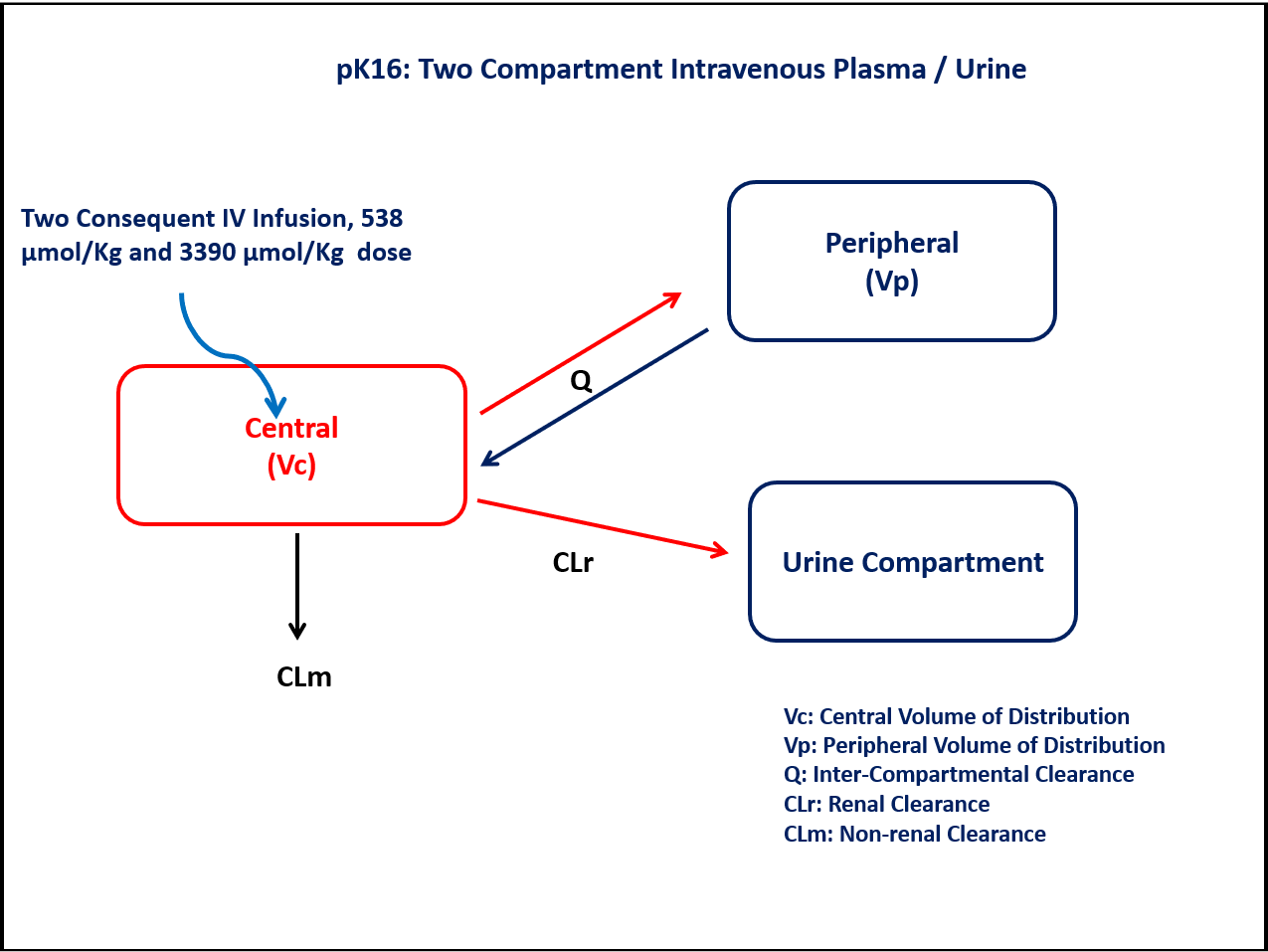
PK16 - Two-compartment intravenous plasma/urine
1 Background
- Structural Model - Two Compartment model with first order elimination
- Route of Administration - Intravenous infusion (Multiple-dose)
- Dosage Regimen - 538 µmol/kg followed by 3390 µmol/kg
- Number of Subjects - 1
2 Learning Outcome
This exercise explains a simultaneous analysis of plasma and urine data using a two-compartment model, with an additional urinary compartment accounting for the amount of drug excreted in urine.
3 Objectives
In this exercise, you will learn how to build a two compartment model and to simulate the data for a single subject based on the given dosage regimen.
4 Libraries
Call the necessary libraries to get started
5 Model
A two-compartment model with one Central and one Peripheral compartment will help in understanding the plasma concentration. A separate Urine compartment accounts for the fraction (amount) of drug excreted in urine.
pk_16 = @model begin
    @metadata begin
        desc = "Two Compartment Model with Urine Compartment"
        timeu = u"hr"
    end

    @param begin
        """
        Renal Clearance (L/hr/kg)
        """
        tvclr ∈ RealDomain(lower = 0)
        """
        Non-renal Clearance (L/hr/kg)
        """
        tvclm ∈ RealDomain(lower = 0)
        """
        Volume of Central Compartment (L/kg)
        """
        tvvc ∈ RealDomain(lower = 0)
        """
        Volume of Peripheral Compartment (L/kg)
        """
        tvvp ∈ RealDomain(lower = 0)
        """
        Inter-compartmental Clearance (L/hr/kg)
        """
        tvq ∈ RealDomain(lower = 0)
        Ω ∈ PDiagDomain(5)
        """
        Proportional RUV - Plasma
        """
        σ₁_prop ∈ RealDomain(lower = 0)
        """
        Proportional RUV - Urine
        """
        σ₂_prop ∈ RealDomain(lower = 0)
    end

    @random begin
        η ~ MvNormal(Ω)
    end

    @pre begin
        CLr = tvclr * exp(η[1])
        CLm = tvclm * exp(η[2])
        Vc = tvvc * exp(η[3])
        Vp = tvvp * exp(η[4])
        Q = tvq * exp(η[5])
        CL = CLr + CLm
        Vss = Vc + Vp
        t12 = 0.693 * Vss / CL
    end

    @dynamics begin
        Central' =
            -(CLr / Vc) * Central - (CLm / Vc) * Central + (Q / Vp) * Peripheral -
            (Q / Vc) * Central
        Peripheral' = (Q / Vc) * Central - (Q / Vp) * Peripheral
        Urine' = (CLr / Vc) * Central
    end

    @derived begin
        cp_plasma = @. Central / (Vc + eps())
        """
        Observed Plasma Concentration (μM)
        """
        dv_plasma ~ @. ProportionalNormal(cp_plasma, σ₁_prop)
        cp_urine = @. Urine
        """
        Observed Urine Amount (μmol)
        """
        dv_urine ~ @. ProportionalNormal(cp_urine, σ₂_prop)
    end
end
┌ Warning: Variable `cp_plasma` is defined in the `@derived` block using `=` and hence `cp_plasma` is not used for model fitting but only returned when simulating: │ If `cp_plasma` is a random variable, it must be defined in the `@derived` block using `~`; │ if `cp_plasma` should be returned when simulating, it should be defined in the `@observed` block using `=`; │ if `cp_plasma` is an intermediate quantity that should not be returned when simulating, it should be defined using `:=`. └ @ Pumas ~/run/_work/PumasTutorials.jl/PumasTutorials.jl/custom_julia_depot/packages/Pumas/GZeMg/src/dsl/model_macro.jl:2351 ┌ Warning: Variable `cp_urine` is defined in the `@derived` block using `=` and hence `cp_urine` is not used for model fitting but only returned when simulating: │ If `cp_urine` is a random variable, it must be defined in the `@derived` block using `~`; │ if `cp_urine` should be returned when simulating, it should be defined in the `@observed` block using `=`; │ if `cp_urine` is an intermediate quantity that should not be returned when simulating, it should be defined using `:=`. └ @ Pumas ~/run/_work/PumasTutorials.jl/PumasTutorials.jl/custom_julia_depot/packages/Pumas/GZeMg/src/dsl/model_macro.jl:2351
PumasModel
  Parameters: tvclr, tvclm, tvvc, tvvp, tvq, Ω, σ₁_prop, σ₂_prop
  Random effects: η
  Covariates:
  Dynamical system variables: Central, Peripheral, Urine
  Dynamical system type: Matrix exponential
  Derived: cp_plasma, dv_plasma, cp_urine, dv_urine
  Observed: cp_plasma, dv_plasma, cp_urine, dv_urine
6 Parameters
CLr- Renal Clearance (L/hr/kg)CLm- Non-renal Clearance (L/hr/kg)Vc- Volume of Central Compartment (L/kg)Vp- Volume of Peripheral Compartment (L/kg)Q- Inter-compartmental Clearance (L/hr/kg)Ω- Between Subject Variabilityσ²₁- Residual error 1 (for plasma conc)σ²₂- Residual error 2 (for amount excreted in urine)
Derived Parameters:
CL- Total Clearance (L/hr/kg)Vss- Volume of distribution at steady state (L/kg)t1/2- Half life (hr)
Typical value (tv) estimates for individual parameters
param = (
    tvclm = 0.05,
    tvclr = 0.31,
    tvvc = 1.6,
    tvvp = 0.16,
    tvq = 0.03,
    Ω = Diagonal([0.04, 0.04, 0.04, 0.04, 0.04]),
    σ₁_prop = 0.1,
    σ₂_prop = 0.1,
)
7 Dosage Regimen
- The subject (male dog) received two consecutive intravenous infusions of a drug.
- The subject received an initial dose of 538 µmol/kg from time 0 to 0.983 hr (rate = 547.304) followed by 3390 µmol/kg dose from time 0.983 to 23.95 hr (rate = 147.603).
- Total infused dose: 3928 µmol/kg.
ev1 = DosageRegimen([538, 3390], time = [0, 0.983], cmt = [1, 1], rate = [547.304, 147.603])2×10 DataFrame
| Row | time | cmt | amt | evid | ii | addl | rate | duration | ss | route |
|---|---|---|---|---|---|---|---|---|---|---|
| Float64 | Int64 | Float64 | Int8 | Float64 | Int64 | Float64 | Float64 | Int8 | NCA.Route | |
| 1 | 0.0 | 1 | 538.0 | 1 | 0.0 | 0 | 547.304 | 0.983 | 0 | NullRoute |
| 2 | 0.983 | 1 | 3390.0 | 1 | 0.0 | 0 | 147.603 | 22.967 | 0 | NullRoute |
sub1 = Subject(id = 1, events = ev1)Subject
ID: 1
Events: 28 Simulation
To simulate the following for the above subject with specific observation time points.
- Plasma concentration.
- Amount excreted unchanged in urine.
Random.seed!(123)The random effects are zero’ed out since we are simulating means
zfx = zero_randeffs(pk_16, sub1, param)(η = [0.0, 0.0, 0.0, 0.0, 0.0],)sim_sub1 = simobs(
pk_16,
sub1,
param,
zfx,
obstimes = [
0.5,
1,
2,
4,
6.1,
7.6,
8.02,
12.05,
12.15,
15.95,
22.13,
23.89,
24.05,
24.46,
24.94,
25.94,
26.96,
27.95,
29.97,
31.94,
35.96,
36.2,
48,
48.2,
54,
60,
60.2,
72,
72.2,
],
)SimulatedObservations
Simulated variables: cp_plasma, dv_plasma, cp_urine, dv_urine
Time: [0.5, 1.0, 2.0, 4.0, 6.1, 7.6, 8.02, 12.05, 12.15, 15.95 … 31.94, 35.96, 36.2, 48.0, 48.2, 54.0, 60.0, 60.2, 72.0, 72.2]9 Visualization
Create a DataFrame of the simulated data.
df1 = DataFrame(sim_sub1)
first(df1, 5)
5×32 DataFrame
| Row | id | time | cp_plasma | dv_plasma | cp_urine | dv_urine | evid | amt | cmt | rate | duration | ss | ii | route | tad | dosenum | Central | Peripheral | Urine | η₁ | η₂ | η₃ | η₄ | η₅ | CLr | CLm | Vc | Vp | Q | CL | Vss | t12 |
|---|---|---|---|---|---|---|---|---|---|---|---|---|---|---|---|---|---|---|---|---|---|---|---|---|---|---|---|---|---|---|---|---|
| String | Float64 | Float64? | Float64? | Float64? | Float64? | Int64? | Float64? | Symbol? | Float64? | Float64? | Int8? | Float64? | NCA.Route? | Float64? | Int64? | Float64? | Float64? | Float64? | Float64? | Float64? | Float64? | Float64? | Float64? | Float64? | Float64? | Float64? | Float64? | Float64? | Float64? | Float64? | Float64? | |
| 1 | 1 | 0.0 | missing | missing | missing | missing | 1 | 538.0 | Central | 547.304 | 0.983 | 0 | 0.0 | NullRoute | 0.0 | 1 | missing | missing | missing | 0.0 | 0.0 | 0.0 | 0.0 | 0.0 | 0.31 | 0.05 | 1.6 | 0.16 | 0.03 | 0.36 | 1.76 | 3.388 |
| 2 | 1 | 0.5 | 161.044 | 197.853 | 12.7335 | 12.8771 | 0 | 0.0 | missing | 0.0 | 0.0 | 0 | 0.0 | missing | 0.5 | 1 | 257.67 | 1.19427 | 12.7335 | 0.0 | 0.0 | 0.0 | 0.0 | 0.0 | 0.31 | 0.05 | 1.6 | 0.16 | 0.03 | 0.36 | 1.76 | 3.388 |
| 3 | 1 | 0.983 | missing | missing | missing | missing | 1 | 3390.0 | Central | 147.603 | 22.967 | 0 | 0.0 | NullRoute | 0.0 | 2 | missing | missing | missing | 0.0 | 0.0 | 0.0 | 0.0 | 0.0 | 0.31 | 0.05 | 1.6 | 0.16 | 0.03 | 0.36 | 1.76 | 3.388 |
| 4 | 1 | 1.0 | 299.498 | 329.475 | 48.9648 | 45.6864 | 0 | 0.0 | missing | 0.0 | 0.0 | 0 | 0.0 | missing | 0.017 | 2 | 479.197 | 4.45023 | 48.9648 | 0.0 | 0.0 | 0.0 | 0.0 | 0.0 | 0.31 | 0.05 | 1.6 | 0.16 | 0.03 | 0.36 | 1.76 | 3.388 |
| 5 | 1 | 2.0 | 317.468 | 324.495 | 144.684 | 143.559 | 0 | 0.0 | missing | 0.0 | 0.0 | 0 | 0.0 | missing | 1.017 | 2 | 507.948 | 12.1436 | 144.684 | 0.0 | 0.0 | 0.0 | 0.0 | 0.0 | 0.31 | 0.05 | 1.6 | 0.16 | 0.03 | 0.36 | 1.76 | 3.388 |
time_plasma = [
    0.5,
    1,
    2,
    4,
    7.6,
    8.02,
    12.05,
    15.95,
    22.13,
    23.89,
    24.46,
    24.94,
    25.94,
    26.96,
    27.95,
    29.97,
    31.94,
    35.96,
    48,
    54,
    60,
    72,
]

df_plasma = @rsubset df1 :time in time_plasma
time_urine = [6.1, 12.15, 24.05, 36.2, 48.2, 60.2, 72.2]
df_urine = @rsubset df1 :time in time_urinePlot the simulated plasma concentration data and the amount of drug excreted in urine in a single plot.
plasma_plt = @chain df_plasma begin
    @rtransform :Matrix = "Plasma"
    data(_) *
    mapping(
        :time => "Time (hours)",
        :cp_plasma => "Concentration (μM) & Amount (μmol)",
        color = :Matrix,
    ) *
    visual(ScatterLines, color = :blue, linewidth = 4)
end

urine_plt = @chain df_urine begin
    @rtransform :Matrix = "Urine"
    data(_) *
    mapping(
        :time => "Time (hours)",
        :cp_urine => "Concentration (μM) & Amount (μmol)",
        color = :Matrix,
    ) *
    visual(ScatterLines, color = :black, linewidth = 4)
end

draw(
    plasma_plt + urine_plt;
    axis = (;
        xticks = [0, 10, 20, 30, 40, 50, 60, 70, 80],
        yticks = [0.1, 0, 1, 10, 100, 1000, 10000],
        yscale = log,
        ytickformat = x -> string.(round.(x; digits = 1)),
        ygridwidth = 3,
        yminorticksvisible = true,
        yminorgridvisible = true,
        yminorticks = IntervalsBetween(10),
        xminorticksvisible = true,
        xminorgridvisible = true,
        xminorticks = IntervalsBetween(5),
    ),
    figure = (; fontsize = 22,),
)
10 Population simulation
par = (
    tvclm = 0.05,
    tvclr = 0.31,
    tvvc = 1.6,
    tvvp = 0.16,
    tvq = 0.03,
    Ω = Diagonal([0.0081, 0.004, 0.0004, 0.0256, 0.0676]),
    σ₁_prop = 0.04,
    σ₂_prop = 0.09,
)

ev1 = DosageRegimen([538, 3390], time = [0, 0.983], cmt = [1, 1], rate = [547.304, 147.603])
pop = map(i -> Subject(id = i, events = ev1), 1:80)

Random.seed!(1234)
pop_sim = simobs(
    pk_16,
    pop,
    par,
    obstimes = [
        0.5,
        1,
        2,
        4,
        6.1,
        7.6,
        8.02,
        12.05,
        15.95,
        22.13,
        23.89,
        24.46,
        24.94,
        25.94,
        26.96,
        27.95,
        29.97,
        31.94,
        36,
        48,
        54,
        60,
        72,
    ],
)

df_sim = DataFrame(pop_sim)
#CSV.write("pk_16.csv", df_sim)