using Pumas
using PumasUtilities
using Random
using CairoMakie
using AlgebraOfGraphics
using CSV
using DataFramesMeta
PK18 - Capacity II - Ethanol kinetics
1 Learning Outcome
In this tutorial, you will learn how to build a two compartment disposition model with non-linear elimination following Intravenous infusion and simulate the model for a single subject and a single dosage regimen.
2 Objectives
In this modeling exercise, you will learn:
- To build a two compartment disposition model. The drug is given as an
Intravenous Infusion, which follows Michaelis-Menten Kinetics. - To apply differential equations in the model as per the compartment model.
- To design the dosage regimen for the subjects and simulate the plot.
3 Background
Before constructing a model, it is important to establish the process the model will follow and a scenario for the simulation.
Below is the scenario for this tutorial:
- Structural model - Two compartment disposition model with nonlinear elimination
- Route of administration - IV infusion
- Dosage Regimen - 0.4 g/kg (i.e., 28 g for a 70 kg healthy individual), infused over a time span of 30 minutes
- Number of Subjects - 1
WarningLook at the dose!
Take note that this tutorial uses a weight-based dosing regimen. You may need to alter your simulation if this is not the scenario of interest in your workflow.
This diagram describes how such an administered dose will be handled, which facilitates building the model. 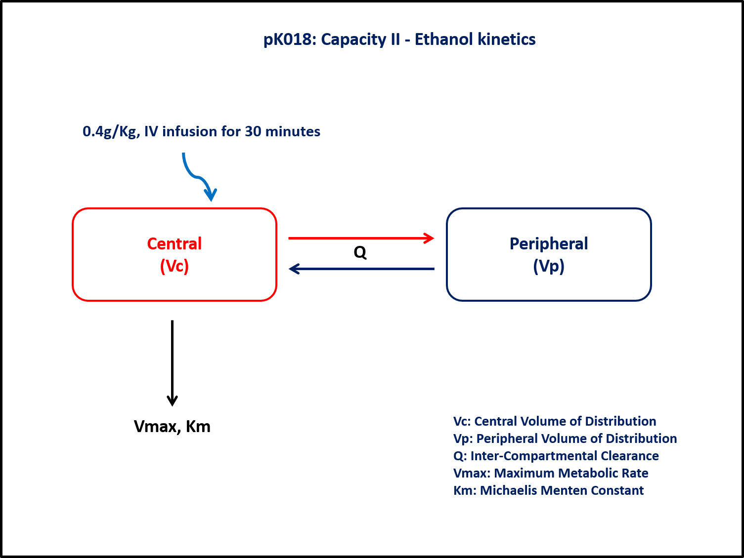
4 Libraries
Call the required libraries to get started.
5 Model
In this two compartment model, we administer a dose on the central compartment.
pk_18 = @model begin
    @metadata begin
        desc = "Two Compartment Model - Nonlinear Elimination"
        timeu = u"hr"
    end

    @param begin
        """
        Maximum rate of elimination (mg/hr)
        """
        tvvmax ∈ RealDomain(lower = 0)
        """
        Michaelis-Menten rate constant (mg/L)
        """
        tvkm ∈ RealDomain(lower = 0)
        """
        Intercompartmental Clearance (L/hr)
        """
        tvQ ∈ RealDomain(lower = 0)
        """
        Volume of Central Compartment (L)
        """
        tvvc ∈ RealDomain(lower = 0)
        """
        Volume of Peripheral Compartment (L)
        """
        tvvp ∈ RealDomain(lower = 0)
        Ω ∈ PDiagDomain(5)
        """
        Proportional RUV
        """
        σ²_prop ∈ RealDomain(lower = 0)
    end

    @random begin
        η ~ MvNormal(Ω)
    end

    @pre begin
        Vmax = tvvmax * exp(η[1])
        Km = tvkm * exp(η[2])
        Q = tvQ * exp(η[3])
        Vc = tvvc * exp(η[4])
        Vp = tvvp * exp(η[5])
    end

    @dynamics begin
        Central' =
            -(Vmax / (Km + (Central / Vc))) * Central / Vc + (Q / Vp) * Peripheral -
            (Q / Vc) * Central
        Peripheral' = -(Q / Vp) * Peripheral + (Q / Vc) * Central
    end

    @derived begin
        cp = @. Central / Vc
        """
        Observed Concentration (g/L)
        """
        dv ~ ProportionalNormal.(cp, sqrt(σ²_prop))
    end
end
┌ Warning: Variable `cp` is defined in the `@derived` block using `=` and hence `cp` is not used for model fitting but only returned when simulating: │ If `cp` is a random variable, it must be defined in the `@derived` block using `~`; │ if `cp` should be returned when simulating, it should be defined in the `@observed` block using `=`; │ if `cp` is an intermediate quantity that should not be returned when simulating, it should be defined using `:=`. └ @ Pumas ~/run/_work/PumasTutorials.jl/PumasTutorials.jl/custom_julia_depot/packages/Pumas/GZeMg/src/dsl/model_macro.jl:2351
PumasModel
  Parameters: tvvmax, tvkm, tvQ, tvvc, tvvp, Ω, σ²_prop
  Random effects: η
  Covariates:
  Dynamical system variables: Central, Peripheral
  Dynamical system type: Nonlinear ODE
  Derived: cp, dv
  Observed: cp, dv
6 Parameters
The compound follows a two compartment model. The parameters are as given below.
Vmax- Maximum rate of elimination (mg/hr)Km- Michaelis-Menten rate constant (mg/L)Q- Intercompartmental Clearance (L/hr)Vc- Volume of Central Compartment (L)Vp- Volume of Peripheral Compartment (L)Ω- Between Subject Variabilityσ- Residual error
These are the initial estimates we will be using in this model exercise. Note that tv represents the typical value for parameters.
param = (;
    tvvmax = 0.0812189,
    tvkm = 0.0125445,
    tvQ = 1.29034,
    tvvc = 8.93016,
    tvvp = 31.1174,
    Ω = Diagonal([0.01, 0.01, 0.01, 0.01, 0.01]),
    σ²_prop = 0.005,
)
7 Dosage Regimen
To start the simulation process, the dosing regimen from the background section must be developed first prior to running a simulation.
The Dosage regimen is specified as:
0.4 g/kg (i.e., 28 g for a 70 kg healthy individual), infused over a time span of 30 minutes, is administered to a single subject.
WarningLook at the dose!
Take note that this tutorial uses a weight-based dosing regimen. You may need to alter your simulation if this is not the scenario of interest in your workflow.
This is how to establish the dosing regimen:
ev1 = DosageRegimen(28; time = 0, cmt = 1, duration = 30)1×10 DataFrame
| Row | time | cmt | amt | evid | ii | addl | rate | duration | ss | route |
|---|---|---|---|---|---|---|---|---|---|---|
| Float64 | Int64 | Float64 | Int8 | Float64 | Int64 | Float64 | Float64 | Int8 | NCA.Route | |
| 1 | 0.0 | 1 | 28.0 | 1 | 0.0 | 0 | 0.933333 | 30.0 | 0 | NullRoute |
This is how to create the single subject undergoing the dosing regimen above.
sub1 = Subject(; id = 1, events = ev1)Subject
ID: 1
Events: 18 Simulation
Let’s simulate for plasma concentration with the specific observation time points after intravenous administration.
NoteRandom.seed!()
The Random.seed! function is included here for purposes of reproducibility of the simulation in this tutorial. Specification of a seed value would not be required in a Pumas workflow that is estimating model parameters.
Random.seed!(1234)sim_sub = simobs(pk_18, sub1, param, obstimes = 0.1:1:360)SimulatedObservations
Simulated variables: cp, dv
Time: 0.1:1.0:359.19 Visualization
Plotting the simulated model predictions:
@chain DataFrame(sim_sub) begin
    dropmissing(:cp)
    data(_) *
    mapping(:time => "Time (hours)", :cp => "Concentration (g/L)") *
    visual(Lines; linewidth = 4)
    draw(;
        figure = (; fontsize = 22),
        axis = (;
            yscale = log10,
            yticks = map(i -> 10.0^i, -2:1),
            ytickformat = i -> (@. string(round(i; digits = 1))),
            xticks = 0:50:400,
        ),
    )
end
The simulation results show a profile that exhibits nonlinear elimination.
10 Population Simulation
This block updates the parameters of the model to increase intersubject variability in parameters and defines timepoints for the predicted of concentrations. The results are written to a CSV file.
par = (
    tvvmax = 0.0812189,
    tvkm = 0.0125445,
    tvQ = 1.29034,
    tvvc = 8.93016,
    tvvp = 31.1174,
    Ω = Diagonal([0.0425, 0.0902, 0.0524, 0.0326, 0.0125]),
    σ²_prop = 0.04,
)

ev1 = DosageRegimen(28; time = 0, cmt = 1, duration = 30)
pop = map(i -> Subject(id = i, events = ev1), 1:55)

Random.seed!(123)
pop_sim = simobs(
    pk_18,
    pop,
    par,
    obstimes = [
        5,
        10,
        15,
        20,
        25,
        30,
        35,
        40,
        45,
        50,
        55,
        60,
        70,
        75,
        80,
        85,
        90,
        95,
        105,
        110,
        115,
        120,
        125,
        130,
        135,
        140,
        145,
        150,
        155,
        160,
        165,
        170,
        175,
        180,
        190,
        195,
        200,
        205,
        210,
        215,
        220,
        225,
        230,
        235,
        240,
        255,
        270,
        285,
        300,
        315,
        330,
        345,
        360,
    ],
)
sim_plot(pop_sim, yaxis = :log, ylims = (0.01, 10))

df_sim = DataFrame(pop_sim)

#CSV.write("pk_18.csv", df_sim)
NoteSaving the Simulation Results
With the CSV.write function, you can input the name of the dataframe (df_sim) and the file name of your choice (pk_18.csv) to save the file to your local directory or repository.
11 Conclusion
In this tutorial, a compound such as Ethanol, which exhibits non-linear elimination, was fitted to a model. Constructing a model such as this involves:
- understanding the process of how the drug is passed through the system,
- quantitatively explaining non-linear kinetics of elimination, and
- simulating the model in a single patient for evaluation.