using PumasUtilities
using Random
using Pumas
using CairoMakie
using AlgebraOfGraphics
using CSV
using DataFramesMeta
using Dates
PK21 - Heteroinduction model
1 Background
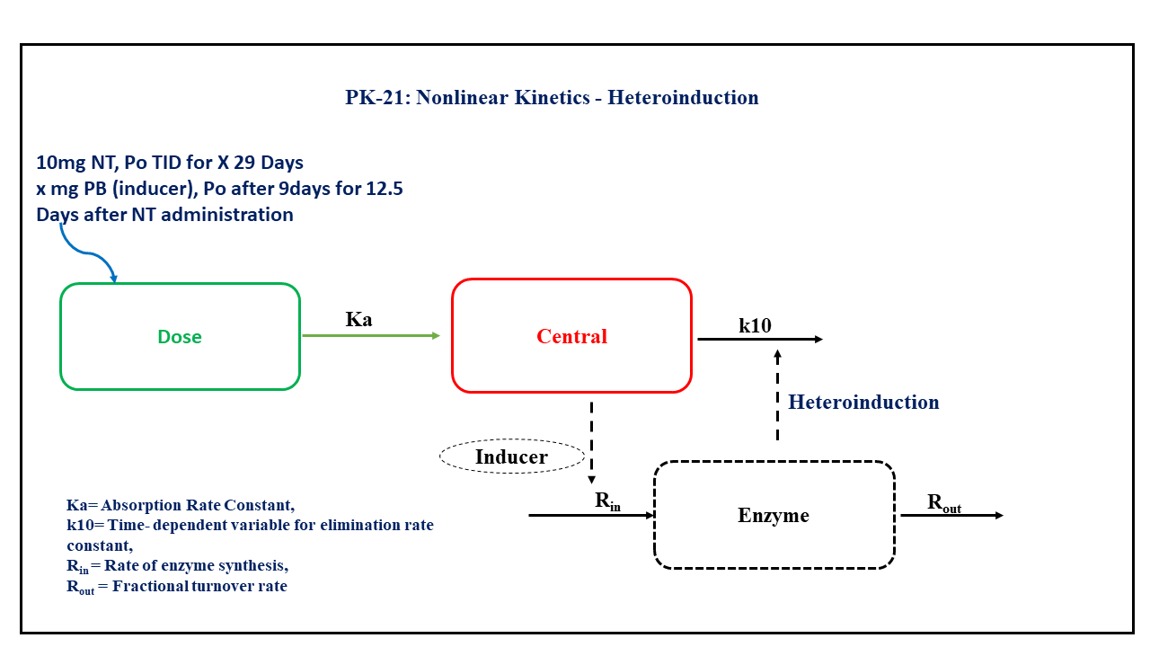
- Structural model - One compartment oral administration consists of time dependent change in the elimination rate constant.
- Route of administration - Oral
- Dosage Regimen - Nortriptyline (NT) 10 mg (or 10000 μg) oral, three times daily for 29 days (i.e., 696 hours), after 216 hours treatment with an enzyme inducer, i.e. Pentobarbital (PB), for a period of 300 hours, i.e., up until 516 hours of treatment with NT.
- Number of Subjects - 1
2 Learning Outcome
This exercise demonstrates simulating from a heteroinduction model after repeated oral doses with an enzyme inducer for a limited duration.
3 Objectives
To build an oral one-compartment model with enzyme induction where clearance is time dependent, simulate the model for a single subject, and subsequently perform simulation for a population.
Certain assumptions are to be considered:
- The fractional turnover rate, i.e.,
Koutof the enzyme has a longer half-life than the drug or the inducer - The duration from one level of enzyme activity to others will be influenced by
Koutof the enzyme - The
Koutis not regulated by the Pentobarbital. The interpretationVincludes bioavailability (i.e., it is reallyV/F).
4 Libraries
Load the necessary libraries.
5 Model definition
Note the expression of the model parameters with helpful comments. The model is expressed with differential equations. Residual variability is a proportional error model.
In this one compartment model, we administer the dose in the Depot compartment at time= 0 that is given every 8 hours for 87 additional doses. A second drug, which is an enzyme inducer (Pentobarbital) is added at 216 hours for 300 hours up to 516 hours of treatment with Nortriptyline.
Note
We do not have concentrations of Pentobarbital and hence it is not included in the model.
pk_21 = @model begin
    @metadata begin
        desc = "Heteroinduction Model"
        timeu = u"hr"
    end

    @param begin
        """
        Absorption Rate Constant (1/hr)
        """
        tvka ∈ RealDomain(lower = 0)
        """
        Intrinsic Clearance post-treatment (L/hr)
        """
        tvclss ∈ RealDomain(lower = 0)
        """
        Lag-time (hrs)
        """
        tvlag ∈ RealDomain(lower = 0)
        """
        Intrinsic Clearance pre-treatment (L/hr)
        """
        tvclpre ∈ RealDomain(lower = 0)
        """
        Fractional turnover rate (1/hr)
        """
        tvkout ∈ RealDomain(lower = 0)
        """
        Volume of distribution (L)
        """
        tvv ∈ RealDomain(lower = 0)
        Ω ∈ PDiagDomain(3)
        """
        Proportional RUV
        """
        σ²_prop ∈ RealDomain(lower = 0)
    end

    @random begin
        η ~ MvNormal(Ω)
    end

    @covariates TBP TBP2

    @pre begin
        Ka = tvka * exp(η[1])
        Clpre = tvclpre * exp(η[3])
        Clss = tvclss * exp(η[2])
        Vc = tvv
        Kout = tvkout
        Kpre = Clpre / Vc
        Kss = Clss / Vc
        Kperi = Kss - (Kss - Kpre) * exp(-Kout * (t - TBP))
        A = Kss - (Kss - Kpre) * exp(-Kout * (TBP2 - TBP))
        Kpost = Kpre - (Kpre - A) * exp(-Kout * (t - TBP2))
        K10 = (t < TBP) * Kpre + (t >= TBP && t < TBP2) * Kperi + (t >= TBP2) * Kpost
    end

    @dosecontrol begin
        lags = (Depot = tvlag,)
    end

    @dynamics begin
        Depot' = -Ka * Depot
        Central' = Ka * Depot - K10 * Central
    end

    @derived begin
        cp = @. (1000 / 263.384) * Central / Vc
        """
        Observed Concentration (nM)
        """
        dv ~ ProportionalNormal.(cp, sqrt(σ²_prop))
    end
end
┌ Warning: Variable `cp` is defined in the `@derived` block using `=` and hence `cp` is not used for model fitting but only returned when simulating: │ If `cp` is a random variable, it must be defined in the `@derived` block using `~`; │ if `cp` should be returned when simulating, it should be defined in the `@observed` block using `=`; │ if `cp` is an intermediate quantity that should not be returned when simulating, it should be defined using `:=`. └ @ Pumas ~/run/_work/PumasTutorials.jl/PumasTutorials.jl/custom_julia_depot/packages/Pumas/GZeMg/src/dsl/model_macro.jl:2351
PumasModel
  Parameters: tvka, tvclss, tvlag, tvclpre, tvkout, tvv, Ω, σ²_prop
  Random effects: η
  Covariates: TBP, TBP2
  Dynamical system variables: Depot, Central
  Dynamical system type: Nonlinear ODE
  Derived: cp, dv
  Observed: cp, dv
6 Initial Estimates of Model Parameters
The model parameters for simulation are as given below. Note that tv represents the typical value for parameters.
Ka- Absorption Rate Constant (1/hr)CLss- Intrinsic Clearance post-treatment (L/hr),tlag- Lag-time (hrs),CLpre- Intrinsic Clearance pre-treatment (L/hr),Kout- Fractional turnover rate (1/hr),V- Volume of distribution (L),Ω- Between Subject Variability,σ- Residual error.
param = (
    tvka = 1.8406,
    tvclss = 114.344,
    tvlag = 0.814121,
    tvclpre = 46.296,
    tvkout = 0.00547243,
    tvv = 1679.4,
    Ω = Diagonal([0.01, 0.01, 0.01]),
    σ²_prop = 0.015,
)
7 Dosage Regimen
Dose regimen - Oral dosing of 10 mg or 10000 μg at time=0 that is given every 8 hours for 87 additional doses for a single subject.
ev1 = DosageRegimen(10000, cmt = 1, time = 0, ii = 8, addl = 87)1×10 DataFrame
| Row | time | cmt | amt | evid | ii | addl | rate | duration | ss | route |
|---|---|---|---|---|---|---|---|---|---|---|
| Float64 | Int64 | Float64 | Int8 | Float64 | Int64 | Float64 | Float64 | Int8 | NCA.Route | |
| 1 | 0.0 | 1 | 10000.0 | 1 | 8.0 | 87 | 0.0 | 0.0 | 0 | NullRoute |
8 Single-individual that receives the defined dose
sub1 = Subject(id = 1, events = ev1, covariates = (TBP = 216, TBP2 = 516))Subject
ID: 1
Events: 88
Covariates: TBP, TBP29 Single-Subject Simulation
Simulate the plasma concentration-time profile with given observation time-points for single subject.
Initialize the random number generator with a seed for reproducibility of the simulation
Random.seed!(123)Define the timepoints at which concentration values will be simulated.
sim_sub1 = simobs(pk_21, sub1, param, obstimes = 0:1:800)SimulatedObservations
Simulated variables: cp, dv
Time: 0:1:80010 Visualize Results
@chain DataFrame(sim_sub1) begin
    dropmissing(:cp)
    data(_) *
    mapping(:time => "Time (hours)", :cp => "Concentration (nM)") *
    visual(Lines; linewidth = 4)
    draw(; figure = (; fontsize = 22), axis = (; xticks = 0:100:800))
end
11 Population Simulation
We perform a population simulation with 48 participants, and simulate concentration values for 72 hours following 6 doses administered every 8 hours.
This code demonstrates how to write the simulated concentrations to a comma separated file (.csv).
param = (
    tvka = 1.8406,
    tvclss = 114.344,
    tvlag = 0.814121,
    tvclpre = 46.296,
    tvkout = 0.00547243,
    tvv = 1679.4,
    Ω = Diagonal([0.0568, 0.0925, 0.0685]),
    σ²_prop = 0.04,
)

ev1 = DosageRegimen(10000, cmt = 1, time = 0, ii = 8, addl = 87)
pop = map(i -> Subject(id = i, events = ev1, covariates = (TBP = 216, TBP2 = 516)), 1:45)

Random.seed!(1234)
sim_pop = simobs(
    pk_21,
    pop,
    param,
    obstimes = [
        0,
        168,
        171,
        172,
        175,
        216,
        360,
        361,
        363,
        365,
        368,
        384,
        432,
        504,
        505,
        507,
        509,
        552,
        600,
        696,
        697,
        699,
        701,
        704,
    ],
)

pkdata_21_sim = DataFrame(sim_pop)
#CSV.write("pk_21_sim.csv", pkdata_21_sim)
12 Conclusion
This tutorial showed how to build and simulate from a heteroinduction model after repeated oral dose data on treatment with an enzyme inducer for a limited duration.