using Random
using Pumas
using PumasUtilities
using AlgebraOfGraphics
using CairoMakie
using CSV
using DataFramesMeta
using Dates
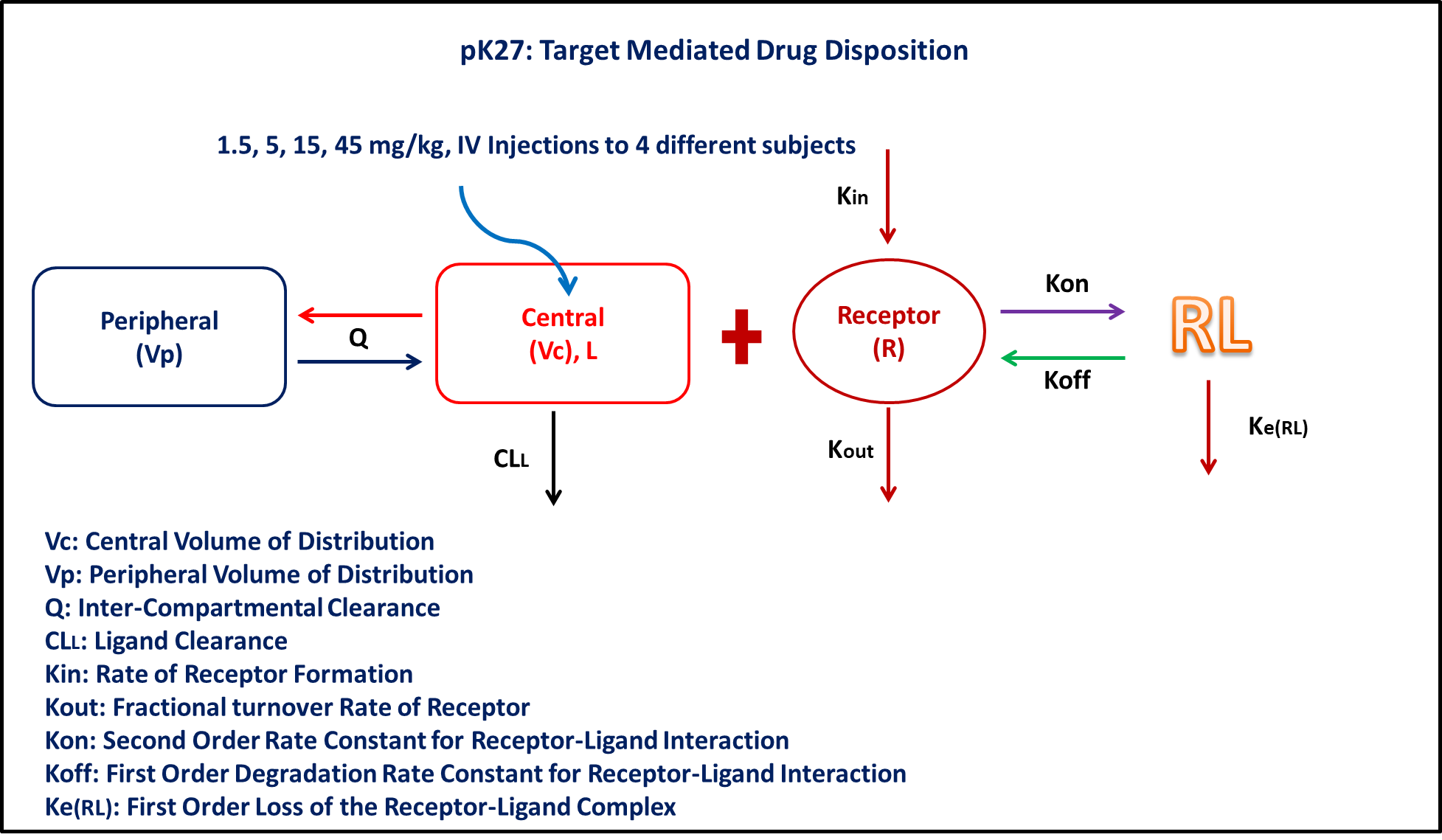
PK27 - Allometry - Elementary & Complex Dedrick plot
1 Background
- Structural model - Target Mediated Drug Disposition Model (TMDD)
- Route of administration - IV-Bolus
- Dosage Regimen - 1.5, 5, 15, 45 mg/kg administered after a complete washout
- Number of Subjects - 4
2 Learning Outcome
- To fit a full TMDD model with data from only ligand, ligand and target, target and ligand-target complex
- Write a differential equation for a full TMDD model
3 Objective
The objective of this exercise is to simulate from a TMDD model
4 Libraries
Call the necessary libraries to get started
5 Model
pk_27 = @model begin
    @metadata begin
        desc = "Target Mediated Drug Disposition Model"
        timeu = u"hr"
    end

    @param begin
        """
        Clearance of central compartment (L/kg/hr)
        """
        tvcl ∈ RealDomain(lower = 0)
        """
        Second order on rate of ligand (L/mg/hr)
        """
        tvkon ∈ RealDomain(lower = 0)
        """
        First order off rate of ligand (1/hr)
        """
        tvkoff ∈ RealDomain(lower = 0)
        """
        Volume of Peripheral Compartment (L/kg)
        """
        tvvp ∈ RealDomain(lower = 0)
        """
        Inter-compartmental clearance (L/kg/hr)
        """
        tvq ∈ RealDomain(lower = 0)
        """
        Zero order receptor synthesis process (mg/L/hr)
        """
        tvkin ∈ RealDomain(lower = 0)
        """
        First order receptor degeneration process (1/hr)
        """
        tvkout ∈ RealDomain(lower = 0)
        """
        First order elimination of complex (1/hr)
        """
        tvkerl ∈ RealDomain(lower = 0)
        """
        Volume of Central Compartment (L/kg)
        """
        tvvc ∈ RealDomain(lower = 0)
        Ω ∈ PDiagDomain(9)
        """
        Proportional RUV - Plasma
        """
        σ²_prop_cp ∈ RealDomain(lower = 0)
        """
        Proportional RUV - Receptor
        """
        σ²_prop_rec ∈ RealDomain(lower = 0)
        """
        Proportional RUV - Complex
        """
        σ²_prop_com ∈ RealDomain(lower = 0)
    end

    @random begin
        η ~ MvNormal(Ω)
    end

    @pre begin
        Cl = tvcl * exp(η[1])
        Kon = tvkon * exp(η[2])
        Koff = tvkoff * exp(η[3])
        Vp = tvvp * exp(η[4])
        Q = tvq * exp(η[5])
        Kin = tvkin * exp(η[6])
        Kout = tvkout * exp(η[7])
        Kerl = tvkerl * exp(η[8])
        Vc = tvvc * exp(η[9])
    end

    @dosecontrol begin
        Vc_ := tvvc * exp(η[9])
        bioav = (Central = 1 / Vc_,)
    end

    @init begin
        Receptor = Kin / Kout
    end

    @dynamics begin
        Central' =
            -(Cl / Vc) * Central - (Q / Vc) * Central + (Q / Vp) * Peripheral -
            Kon * Receptor * Central + Koff * Complex
        Peripheral' = (Q / Vc) * Central - (Q / Vp) * Peripheral
        Receptor' = Kin - Kout * Receptor - Kon * Receptor * Central + Koff * Complex
        Complex' = Kon * Receptor * Central - Koff * Complex - Kerl * Complex
    end

    @derived begin
        cp = @. Central
        """
        Observed Concentration - Plasma (mg/L)
        """
        dv_cp ~ ProportionalNormal.(cp, sqrt(σ²_prop_cp))
        rec = @. Receptor
        """
        Observed Concentration - Receptor (mg/L)
        """
        dv_rec ~ ProportionalNormal.(rec, sqrt(σ²_prop_rec))
        com = @. Complex
        """
        Observed Concentration - Complex (mg/L)
        """
        dv_com ~ ProportionalNormal.(com, sqrt(σ²_prop_com))
    end
end
┌ Warning: Variable `cp` is defined in the `@derived` block using `=` and hence `cp` is not used for model fitting but only returned when simulating: │ If `cp` is a random variable, it must be defined in the `@derived` block using `~`; │ if `cp` should be returned when simulating, it should be defined in the `@observed` block using `=`; │ if `cp` is an intermediate quantity that should not be returned when simulating, it should be defined using `:=`. └ @ Pumas ~/run/_work/PumasTutorials.jl/PumasTutorials.jl/custom_julia_depot/packages/Pumas/qxx5c/src/dsl/model_macro.jl:2351 ┌ Warning: Variable `rec` is defined in the `@derived` block using `=` and hence `rec` is not used for model fitting but only returned when simulating: │ If `rec` is a random variable, it must be defined in the `@derived` block using `~`; │ if `rec` should be returned when simulating, it should be defined in the `@observed` block using `=`; │ if `rec` is an intermediate quantity that should not be returned when simulating, it should be defined using `:=`. └ @ Pumas ~/run/_work/PumasTutorials.jl/PumasTutorials.jl/custom_julia_depot/packages/Pumas/qxx5c/src/dsl/model_macro.jl:2351 ┌ Warning: Variable `com` is defined in the `@derived` block using `=` and hence `com` is not used for model fitting but only returned when simulating: │ If `com` is a random variable, it must be defined in the `@derived` block using `~`; │ if `com` should be returned when simulating, it should be defined in the `@observed` block using `=`; │ if `com` is an intermediate quantity that should not be returned when simulating, it should be defined using `:=`. └ @ Pumas ~/run/_work/PumasTutorials.jl/PumasTutorials.jl/custom_julia_depot/packages/Pumas/qxx5c/src/dsl/model_macro.jl:2351
PumasModel
  Parameters: tvcl, tvkon, tvkoff, tvvp, tvq, tvkin, tvkout, tvkerl, tvvc, Ω, σ²_prop_cp, σ²_prop_rec, σ²_prop_com
  Random effects: η
  Covariates:
  Dynamical system variables: Central, Peripheral, Receptor, Complex
  Dynamical system type: Nonlinear ODE
  Derived: cp, dv_cp, rec, dv_rec, com, dv_com
  Observed: cp, dv_cp, rec, dv_rec, com, dv_com
6 Parameters
The parameters are as given below. tv represents the typical value for parameters.
Cl- Clearance of central compartment (L/kg/hr)Kon- Second order on rate of ligand (L/mg/hr)Koff- First order off rate of ligand (1/hr)Vp- Volume of Peripheral Compartment (L/kg)Q- Inter-compartmental clearance (L/kg/hr)Kin- Zero order receptor synthesis process (mg/L/hr)Kout- First order receptor degeneration process (1/hr)Kerl- First order elimination of complex (1/hr)Vc- Volume of Central Compartment (L/kg)
param = (
    tvcl = 0.001,
    tvkon = 0.096,
    tvkoff = 0.001,
    tvvp = 0.100,
    tvq = 0.003,
    tvkin = 0.11,
    tvkout = 0.0089,
    tvkerl = 0.003,
    tvvc = 0.05,
    Ω = Diagonal([0.04, 0.04, 0.04, 0.04, 0.04, 0.04, 0.04, 0.04, 0.04]),
    σ²_prop_cp = 0.02,
    σ²_prop_rec = 0.012,
    σ²_prop_com = 0.015,
)
7 Dosage Regimen
- Single dose of 1.5 mg/kg was administered as IV-Bolus at
time=0 - Single dose of 5 mg/kg was administered as IV-Bolus at
time=0 - Single dose of 15 mg/kg was administered as IV-Bolus at
time=0 - Single dose of 45 mg/kg was administered as IV-Bolus at
time=0
dose = [1.5, 5, 15, 45]ids = ["1.5 mg/kg", "5 mg/kg", "15 mg/kg", "45 mg/kg"]dose_ind(x) = DosageRegimen(dose[x], time = 0, cmt = 1)pop4_sub = map(i -> Subject(id = ids[i], events = dose_ind(i)), 1:length(ids))Population
Subjects: 4
Observations: 8 Simulation
Random.seed!(123)The random effects are zero’ed out since we are simulating means
zfx = zero_randeffs(pk_27, pop4_sub, param)4-element Vector{@NamedTuple{η::Vector{Float64}}}:
(η = [0.0, 0.0, 0.0, 0.0, 0.0, 0.0, 0.0, 0.0, 0.0],)
(η = [0.0, 0.0, 0.0, 0.0, 0.0, 0.0, 0.0, 0.0, 0.0],)
(η = [0.0, 0.0, 0.0, 0.0, 0.0, 0.0, 0.0, 0.0, 0.0],)
(η = [0.0, 0.0, 0.0, 0.0, 0.0, 0.0, 0.0, 0.0, 0.0],)sim_pop4 = simobs(pk_27, pop4_sub, param, zfx, obstimes = 0.1:1:500)Simulated population (Vector{<:Subject})
Simulated subjects: 4
Simulated variables: cp, dv_cp, rec, dv_rec, com, dv_com9 Visualization
df27 = @chain DataFrame(sim_pop4) begin
    dropmissing([:cp, :rec, :com])
end
fig = Figure(; fontsize = 32, resolution = (1200, 1200))
ytickformater(ticks) = @. string(round(ticks; digits = 1))
gridpos = fig[1, 1]
plt1 =
data(df27) *
mapping(
:time => "Time (days)",
:cp => "PK27 Concentrations (mg/L)",
color = :id => nonnumeric => "Doses",
) *
visual(Lines, linewidth = 6)
draw!(
gridpos,
plt1;
axis = (;
title = "Ligand",
yscale = log10,
yticks = map(i -> 10.0^i, -2:2),
ytickformat = ytickformater,
xticks = 0:100:500,
),
)
gridpos = fig[1, 2]
plt2 =
data(df27) *
mapping(
:time => "Time (days)",
:rec => "PK27 Concentrations (mg/L)",
color = :id => nonnumeric => "Doses",
) *
visual(Lines, linewidth = 6)
draw!(
gridpos,
plt2;
axis = (;
title = "Receptor",
yscale = log10,
yticks = map(i -> 10.0^i, -2:1),
ytickformat = ytickformater,
xticks = 0:100:500,
),
)
gridpos = fig[2, 1]
plt3 =
data(df27) *
mapping(
:time => "Time (days)",
:com => "PK27 Concentrations (mg/L)",
color = :id => nonnumeric => "Doses",
) *
visual(Lines, linewidth = 6)
p3 = draw!(
gridpos,
plt3;
axis = (;
title = "Complex",
yscale = log10,
yticks = map(i -> 10.0^i, 0.6:0.2:1.4),
ytickformat = ytickformater,
xticks = 0:100:500,
),
)
gridpos = fig[2, 2]
legend!(
gridpos,
p3;
linewidth = 8,
tellwidth = false,
halign = :right,
valign = :center,
margin = (10, 10, 10, 10),
)
fig┌ Warning: Found `resolution` in the theme when creating a `Scene`. The `resolution` keyword for `Scene`s and `Figure`s has been deprecated. Use `Figure(; size = ...` or `Scene(; size = ...)` instead, which better reflects that this is a unitless size and not a pixel resolution. The key could also come from `set_theme!` calls or related theming functions. └ @ Makie ~/run/_work/PumasTutorials.jl/PumasTutorials.jl/custom_julia_depot/packages/Makie/Vn16E/src/scenes.jl:264

10 Population simulation
par = (
    tvcl = 0.001,
    tvkon = 0.096,
    tvkoff = 0.001,
    tvvp = 0.100,
    tvq = 0.003,
    tvkin = 0.11,
    tvkout = 0.0089,
    tvkerl = 0.003,
    tvvc = 0.05,
    Ω = Diagonal([0.09, 0.04, 0.0125, 0.04, 0.0326, 0.0525, 0.0124, 0.0111, 0.0234]),
    σ²_prop_cp = 0.025,
    σ²_prop_rec = 0.03,
    σ²_prop_com = 0.04,
)

ev1 = DosageRegimen(1.5, cmt = 1, time = 0)
pop1 = map(i -> Subject(id = i, events = ev1), 1:20)
ev2 = DosageRegimen(5, cmt = 1, time = 0)
pop2 = map(i -> Subject(id = i, events = ev2), 21:40)
ev3 = DosageRegimen(15, cmt = 1, time = 0)
pop3 = map(i -> Subject(id = i, events = ev3), 41:60)
ev4 = DosageRegimen(45, cmt = 1, time = 0)
pop4 = map(i -> Subject(id = i, events = ev4), 61:80)
pop = [pop1; pop2; pop3; pop4]

## Simulation
Random.seed!(1234)
sim_pop = simobs(pk_27, pop, par, obstimes = [0.1, 1, 10, 24, 72, 120, 168, 240, 360, 499])
sim_plot(sim_pop)

df_sim = DataFrame(sim_pop);

#CSV.write("pk_27.csv", df_sim)