using Random
using Pumas
using PumasUtilities
using CairoMakie
using AlgebraOfGraphics
using DataFramesMeta
using AlgebraOfGraphics
using CSV
PK28 - Allometry - Elementary Dedrick Plot
1 Learning Outcome
- To learn about Allometry - Elementary Dedrick Plots
- To simultaneously simulate an allometric model to concentration-time data obtained from three different species
2 Background
Before constructing a model, it is important to establish the process the model will follow and a scenario for the simulation.
Below is the scenario for this tutorial:
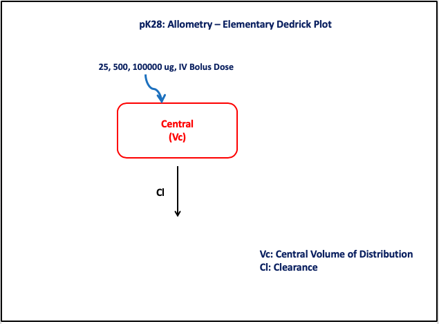
- Structural model - One Compartment Model with Linear Elimination
- Route of administration - IV-Bolus
- Dosage Regimen - 25, 500, 100000 μg administered after complete washout
- Number of Subjects - 3 species (Mouse, Rat, Human)
This diagram describes how such these administered doses will be handled, which facilitates building the model.
3 Libraries
Call the required libraries to get started:
4 Model
The given data follows a one-compartment model with linear elimination
pk_28 = @model begin
    @metadata begin
        desc = "One Compartment Model"
        timeu = u"hr"
    end

    @param begin
        """
        Clearance (L/hr)
        """
        a ∈ RealDomain(lower = 0)
        """
        Scaling parameter for Cl
        """
        b ∈ RealDomain(lower = 0)
        """
        Volume of Distribution (L)
        """
        c ∈ RealDomain(lower = 0)
        """
        Scaling parameter for Vc
        """
        d ∈ RealDomain(lower = 0)
        Ω ∈ PDiagDomain(2)
        """
        proportional RUV
        """
        σ²_prop ∈ RealDomain(lower = 0)
    end

    @random begin
        η ~ MvNormal(Ω)
    end

    @covariates BW

    @pre begin
        Cl = a * (BW)^b * exp(η[1])
        Vc = c * (BW)^d * exp(η[2])
    end

    @dynamics begin
        Central' = -(Cl / Vc) * Central
    end

    @derived begin
        cp = @. Central / Vc
        """
        Observed Concentration (μg/L)
        """
        dv ~ @. Normal(cp, sqrt(cp^2 * σ²_prop))
    end
end
PumasModel
Parameters: a, b, c, d, Ω, σ²_prop
Random effects: η
Covariates: BW
Dynamical system variables: Central
Dynamical system type: Matrix exponential
Derived: cp, dv
Observed: cp, dv5 Parameters
The initial parameters for estimation are given below.
a- typical value of clearance among the speciesb- scaling parameter forClc- typical value of the volume of distribution among the speciesd- scaling parameter forVc
param = (;
    a = 0.319142230070251,
    b = 0.636711976371785,
    c = 3.07665859278123,
    d = 1.03093780182922,
    Ω = Diagonal([0.01, 0.01]),
    σ²_prop = 0.01,
)
6 Dosage Regimen
To start the simulation process, the dosing regimen specified in the background section must be developed first prior to running a simulation.
The Dosage regimen is specified as:
- Species 1 (Mouse) - 25 μg IV-Bolus and bodyweight (23 grams)
- Species 2 (Rat) - 500 μg IV-Bolus and bodyweight (250 grams)
- Species 3 (Human) - 100000 μg IV-Bolus and bodyweight (70 kg)
This represents how to code a dosing event:
ev1 = DosageRegimen(25; cmt = 1, time = 0, route = NCA.IVBolus)1×10 DataFrame
| Row | time | cmt | amt | evid | ii | addl | rate | duration | ss | route |
|---|---|---|---|---|---|---|---|---|---|---|
| Float64 | Int64 | Float64 | Int8 | Float64 | Int64 | Float64 | Float64 | Int8 | NCA.Route | |
| 1 | 0.0 | 1 | 25.0 | 1 | 0.0 | 0 | 0.0 | 0.0 | 0 | IVBolus |
This represents how to code a specific subject. Since the first species is a mouse, id will be "Mouse":
sub1 = Subject(;
    id = "Mouse",
    events = ev1,
    covariates = (BW = 0.023, dose = 25),
    time = [0, 0.167, 0.5, 2, 4, 6],
)
Subject
ID: Mouse
Events: 1
Covariates: BW, doseThe above two steps are repeated for the other species.
ev2 = DosageRegimen(500; cmt = 1, time = 0, route = NCA.IVBolus)1×10 DataFrame
| Row | time | cmt | amt | evid | ii | addl | rate | duration | ss | route |
|---|---|---|---|---|---|---|---|---|---|---|
| Float64 | Int64 | Float64 | Int8 | Float64 | Int64 | Float64 | Float64 | Int8 | NCA.Route | |
| 1 | 0.0 | 1 | 500.0 | 1 | 0.0 | 0 | 0.0 | 0.0 | 0 | IVBolus |
sub2 = Subject(;
    id = "Rat",
    events = ev2,
    covariates = (BW = 0.250, dose = 500),
    time = [0, 0.167, 0.33, 0.5, 1, 2, 4, 8, 12, 15],
)
Subject
ID: Rat
Events: 1
Covariates: BW, doseev3 = DosageRegimen(100000; cmt = 1, time = 0, route = NCA.IVBolus)1×10 DataFrame
| Row | time | cmt | amt | evid | ii | addl | rate | duration | ss | route |
|---|---|---|---|---|---|---|---|---|---|---|
| Float64 | Int64 | Float64 | Int8 | Float64 | Int64 | Float64 | Float64 | Int8 | NCA.Route | |
| 1 | 0.0 | 1 | 100000.0 | 1 | 0.0 | 0 | 0.0 | 0.0 | 0 | IVBolus |
sub3 = Subject(;
    id = "Human",
    events = ev3,
    covariates = (BW = 70, dose = 100000),
    time = [0, 1, 2, 4, 8, 12, 24, 36, 48, 72],
)
Subject
ID: Human
Events: 1
Covariates: BW, doseA population is created with mouse, rat, and human species.
pop3_sub = [sub1, sub2, sub3]If in the event a simulation population’s contents must be inspected, a Pumas user can convert the population to a DataFrame using the DataFrame constructor as shown here:
df_pop3_sub = DataFrame(pop3_sub)
first(df_pop3_sub, 5)
5×14 DataFrame
| Row | id | time | evid | amt | cmt | rate | duration | ss | ii | route | BW | dose | tad | dosenum |
|---|---|---|---|---|---|---|---|---|---|---|---|---|---|---|
| String | Float64 | Int8 | Float64? | Int64? | Float64? | Float64? | Int8? | Float64? | NCA.Route? | Float64? | Int64? | Float64 | Int64 | |
| 1 | Mouse | 0.0 | 0 | 0.0 | missing | 0.0 | 0.0 | 0 | 0.0 | missing | 0.023 | 25 | 0.0 | 1 |
| 2 | Mouse | 0.0 | 1 | 25.0 | 1 | 0.0 | 0.0 | 0 | 0.0 | IVBolus | 0.023 | 25 | 0.0 | 1 |
| 3 | Mouse | 0.167 | 0 | 0.0 | missing | 0.0 | 0.0 | 0 | 0.0 | missing | 0.023 | 25 | 0.167 | 1 |
| 4 | Mouse | 0.5 | 0 | 0.0 | missing | 0.0 | 0.0 | 0 | 0.0 | missing | 0.023 | 25 | 0.5 | 1 |
| 5 | Mouse | 2.0 | 0 | 0.0 | missing | 0.0 | 0.0 | 0 | 0.0 | missing | 0.023 | 25 | 2.0 | 1 |
7 Simulation
Since the model is created and the initial parameters are specified, one should evaluate the model. Simulating with a single subject and population is one way to address this.
Random.seed!()
The Random.seed! function is included here for purposes of reproducibility of the simulation in this tutorial. Specification of a seed value would not be required in a Pumas workflow that is estimating model parameters.
Random.seed!(123)Here, the population is being simulated through simobs which takes the following arguments:
- Model:
pk28 - Simulation Population:
pop3_sub - Initial Parameters:
param
sim_pop3 = simobs(pk_28, pop3_sub, param)Simulated population (Vector{<:Subject})
Simulated subjects: 3
Simulated variables: cp, dv8 Visualization
This is how a Pumas user can generate a plot of Concentration vs Time data from the three different species:
@chain DataFrame(sim_pop3) begin
    dropmissing(:cp)
    data(_) *
    mapping(
        :time => "Time (days)",
        :cp => "Concentration (μg/L)",
        color = :id => "Species",
    ) *
    visual(Lines; linewidth = 4)
    draw(;
        figure = (; fontsize = 22),
        axis = (;
            xticks = 0:10:70,
            yscale = log10,
            yticks = map(i -> 10.0^i, 1:0.5:3),
            ytickformat = i -> (@. string(round(i; digits = 1))),
        ),
    )
end
An Elementary-Dedrick Plot of dose and bodyweight normalized plasma concentration vs bodyweight normalized time can be generated through the following steps:
- Process the data to calculate the x and y-specific factors:
pk28df = @chain sim_pop3 begin
    DataFrame
    @rtransform @passmissing :dv = round(:dv, sigdigits = 2)
    @rtransform @passmissing :amt_bw = :dose / :BW
    @rtransform @passmissing :yfactor = :dv / :amt_bw
    @rtransform @passmissing :bw_b = :BW^(1 - 0.636)
    @rtransform @passmissing :xfactor = :time / :bw_b
    dropmissing!(:dv)
end

first(pk28df, 5)
5×25 DataFrame
| Row | id | time | cp | dv | evid | amt | cmt | rate | duration | ss | ii | route | BW | dose | tad | dosenum | Central | Cl | Vc | η_1 | η_2 | amt_bw | yfactor | bw_b | xfactor |
|---|---|---|---|---|---|---|---|---|---|---|---|---|---|---|---|---|---|---|---|---|---|---|---|---|---|
| String | Float64 | Float64? | Float64 | Int64 | Float64? | Symbol? | Float64? | Float64? | Int8? | Float64? | NCA.Route? | Float64? | Int64? | Float64 | Int64 | Float64? | Float64? | Float64? | Float64 | Float64 | Float64 | Float64? | Float64 | Float64 | |
| 1 | Mouse | 0.0 | 359.21 | 370.0 | 0 | 0.0 | missing | 0.0 | 0.0 | 0 | 0.0 | missing | 0.023 | 25 | 0.0 | 1 | 25.0 | 0.0363197 | 0.0695971 | 0.228566 | 0.100091 | 1086.96 | 0.3404 | 0.25332 | 0.0 |
| 2 | Mouse | 0.167 | 329.23 | 350.0 | 0 | 0.0 | missing | 0.0 | 0.0 | 0 | 0.0 | missing | 0.023 | 25 | 0.167 | 1 | 22.9135 | 0.0363197 | 0.0695971 | 0.228566 | 0.100091 | 1086.96 | 0.322 | 0.25332 | 0.659246 |
| 3 | Mouse | 0.5 | 276.713 | 310.0 | 0 | 0.0 | missing | 0.0 | 0.0 | 0 | 0.0 | missing | 0.023 | 25 | 0.5 | 1 | 19.2584 | 0.0363197 | 0.0695971 | 0.228566 | 0.100091 | 1086.96 | 0.2852 | 0.25332 | 1.97379 |
| 4 | Mouse | 2.0 | 126.494 | 130.0 | 0 | 0.0 | missing | 0.0 | 0.0 | 0 | 0.0 | missing | 0.023 | 25 | 2.0 | 1 | 8.80363 | 0.0363197 | 0.0695971 | 0.228566 | 0.100091 | 1086.96 | 0.1196 | 0.25332 | 7.89516 |
| 5 | Mouse | 4.0 | 44.5443 | 42.0 | 0 | 0.0 | missing | 0.0 | 0.0 | 0 | 0.0 | missing | 0.023 | 25 | 4.0 | 1 | 3.10016 | 0.0363197 | 0.0695971 | 0.228566 | 0.100091 | 1086.96 | 0.03864 | 0.25332 | 15.7903 |
Create the plot:
plt =
    data(pk28df) *
    mapping(
        :xfactor => "Kallynochrons ( h / (BW^(1-b))",
        :yfactor => "Conc / (Dose/BW)",
        color = :id => "Species",
    ) *
    visual(Lines, linewidth = 4)
draw(
    plt;
    figure = (; fontsize = 22),
    axis = (;
        yscale = log10,
        yticks = map(i -> 10.0^i, -2:0.5:1),
        ytickformat = i -> (@. string(round(i; digits = 1))),
        xticks = 0:2:24,
    ),
)
9 Population Simulation
This block updates the parameters of the model to increase intersubject variability in parameters and defines timepoints for prediction of concentrations. The results are written to a CSV file.
par = (
    a = 0.319142230070251,
    b = 0.636711976371785,
    c = 3.07665859278123,
    d = 1.03093780182922,
    Ω = Diagonal([0.0625, 0.0489]),
    σ²_prop = 0.0787759250168089,
)

ev1 = DosageRegimen(25; cmt = 1, time = 0, route = NCA.IVBolus)
pop1 = map(
    i -> Subject(
        id = i,
        events = ev1,
        covariates = (BW = 0.023, Species = "Mouse"),
        time = [0, 0.167, 0.5, 2, 4, 6],
    ),
    1:16,
)
ev2 = DosageRegimen(500; cmt = 1, time = 0, route = NCA.IVBolus)
pop2 = map(
    i -> Subject(
        id = i,
        events = ev2,
        covariates = (BW = 0.250, Species = "Rat"),
        time = [0, 0.167, 0.33, 0.5, 1, 2, 4, 8, 12, 15],
    ),
    17:32,
)
ev3 = DosageRegimen(100000; cmt = 1, time = 0, route = NCA.IVBolus)
pop3 = map(
    i -> Subject(
        id = i,
        events = ev3,
        covariates = (BW = 70, Species = "Human"),
        time = [0, 1, 2, 4, 8, 12, 24, 36, 48, 72],
    ),
    33:48,
)
pop = [pop1; pop2; pop3]

Random.seed!(1234)
sim_pop = simobs(pk_28, pop, par)

df_sim = DataFrame(sim_pop)

#CSV.write("pk_28.csv", df_sim)
Saving the Simulation Results
With the CSV.write function, you can input the name of the DataFrame (df_sim) and the file name of your choice (pk_28.csv) to save the file to your local directory or repository.
10 Conclusion
Constructing a Elementary Dendrick Plot involves:
- understanding the process of how the drug is passed through the system,
- translating processes into ODEs using Pumas,
- preparing the data using Pumas data wrangling functionality, and
- simulating the model in a single patient for evaluation.