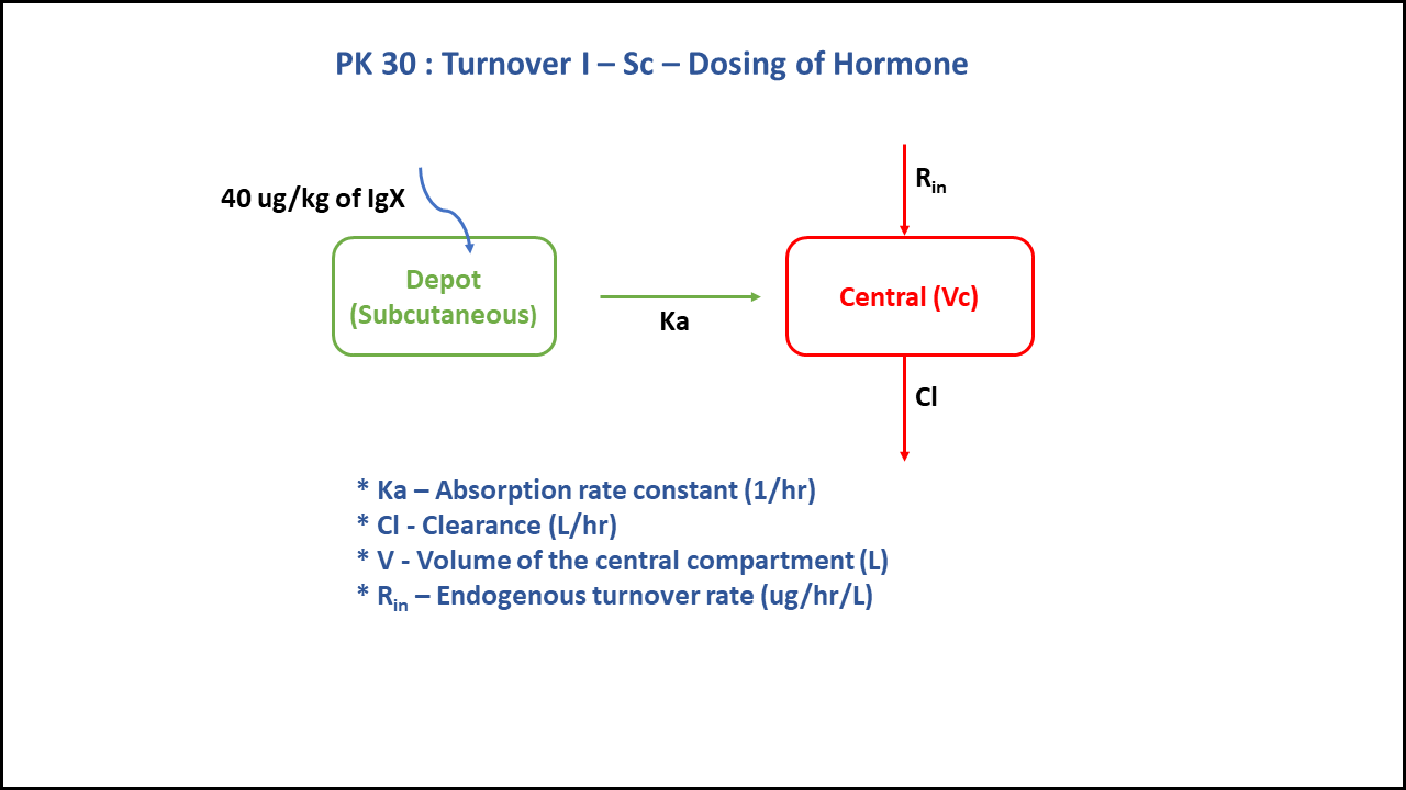
PK30 - Turnover I - SC Dosing of Hormone

1 Background

• Structural model - One compartment first order elimination with zero order production of hormone
• Route of administration - Subcutaneous
• Dosage Regimen - 40 mcg/kg
• Number of Subjects - 1

PK30 Graphic Model

2 Learning Outcome

With subcutaneous dose information, we learn to discriminate between the clearance and the rate of synthesis. Further simplification of the model is done by assuming bioavailability is 100% and concentration of the endogenous compound equals concentration at baseline (turnover/clearance)

3 Objectives

In this tutorial, you will learn how to build a one compartment PK turnover model, following first order elimination kinetics and zero order hormone production.

4 Libraries

Call the necessary libraries to get started

using Random
using Pumas
using PumasUtilities
using CairoMakie
using AlgebraOfGraphics
using CSV
using DataFramesMeta
using Dates

5 Model

In this two compartment model, we administer The dose subcutaneously.

pk_30 = @model begin
    @metadata begin
        desc = "Two Compartment Model"
        timeu = u"hr"
    end

    @param begin
        """
        Absorption rate constant (hr⁻¹)
        """
        tvka ∈ RealDomain(lower = 0)
        """
        Clearance (L/kg/hr)
        """
        tvcl ∈ RealDomain(lower = 0)
        """
        Turnover Rate (hr⁻¹)
        """
        tvsynthesis ∈ RealDomain(lower = 0)
        """
        Volume of Central Compartment (L/kg)
        """
        tvv ∈ RealDomain(lower = 0)
        Ω ∈ PDiagDomain(4)
        """
        Additive RUV
        """
        σ_add ∈ RealDomain(lower = 0)
    end

    @random begin
        η ~ MvNormal(Ω)
    end

    @pre begin
        Ka = tvka * exp(η[1])
        Cl = tvcl * exp(η[2])
        Synthesis = tvsynthesis * exp(η[3])
        V = tvv * exp(η[4])
    end

    @init begin
        Central = Synthesis / (Cl / V) # Concentration at Baseline = Turnover Rate (0.78) / Cl of hormone (0.028)
    end

    @dynamics begin
        Depot' = -Ka * Depot
        Central' = Ka * Depot + Synthesis - (Cl / V) * Central
    end

    @derived begin
        cp = @. Central / V
        """
        Observed Concentration (mcg/L)
        """
        dv ~ @. Normal(cp, σ_add)
    end
end

PumasModel
  Parameters: tvka, tvcl, tvsynthesis, tvv, Ω, σ_add
  Random effects: η
  Covariates:
  Dynamical system variables: Depot, Central
  Dynamical system type: Matrix exponential
  Derived: cp, dv
  Observed: cp, dv

6 Parameters

The parameters are given below. Note that tv represents the typical value for parameters.

• Ka - Absorption rate constant (hr⁻¹)
• Cl - Clearance (L/kg/hr)
• Synthesis - Turnover Rate (hr⁻¹)
• V - Volume of Central Compartment (L/kg)
• Ω - Between Subject Variability
• σ - Residual error

param = (
    tvka = 0.539328,
    tvcl = 0.0279888,
    tvsynthesis = 0.781398,
    tvv = 0.10244,
    Ω = Diagonal([0.04, 0.04, 0.04, 0.04]),
    σ_add = 3.97427,
)

7 Dosage Regimen

A dose of 40 mcg/kg is given subcutaneously to a single subject.

ev1 = DosageRegimen(40, time = 0, cmt = 1)

1×10 DataFrame

Row	time	cmt	amt	evid	ii	addl	rate	duration	ss	route
	Float64	Int64	Float64	Int8	Float64	Int64	Float64	Float64	Int8	NCA.Route
1	0.0	1	40.0	1	0.0	0	0.0	0.0	0	NullRoute

sub1 = Subject(id = 1, events = ev1)

Subject
  ID: 1
  Events: 1

8 Simulation

To simulate plasma concentration with turnover rate after oral administration.

Random.seed!(1234)

The random effects are zero’ed out since we are simulating a single subject

zfx = zero_randeffs(pk_30, sub1, param)

(η = [0.0, 0.0, 0.0, 0.0],)

sim_sub1 = simobs(pk_30, sub1, param, zfx, obstimes = 0:0.1:72)

SimulatedObservations
  Simulated variables: cp, dv
  Time: 0.0:0.1:72.0

9 Visualization

@chain DataFrame(sim_sub1) begin
    dropmissing(:cp)
    data(_) *
    mapping(:time => "Time (hours)", :cp => "Concentration (μg/L)") *
    visual(Lines; linewidth = 4)
    draw(;
        figure = (; fontsize = 22),
        axis = (;
            yscale = log10,
            ytickformat = i -> (@. string(round(i; digits = 1))),
            xticks = 0:10:80,
        ),
    )
end

10 Population simulation

par = (
    tvka = 0.539328,
    tvcl = 0.0279888,
    tvsynthesis = 0.781398,
    tvv = 0.10244,
    Ω = Diagonal([0.0425, 0.0263, 0.0158, 0.0623]),
    σ_add = 3.97427,
)


ev1 = DosageRegimen(40, time = 0, cmt = 1)
pop = map(i -> Subject(id = i, events = ev1), 1:50)

Random.seed!(1234)
pop_sim = simobs(pk_30, pop, par, obstimes = [0, 2, 3, 4, 5, 6, 8, 10, 15, 24, 32, 48, 72])

df_sim = DataFrame(pop_sim)
#CSV.write("pk_30.csv", df_sim)