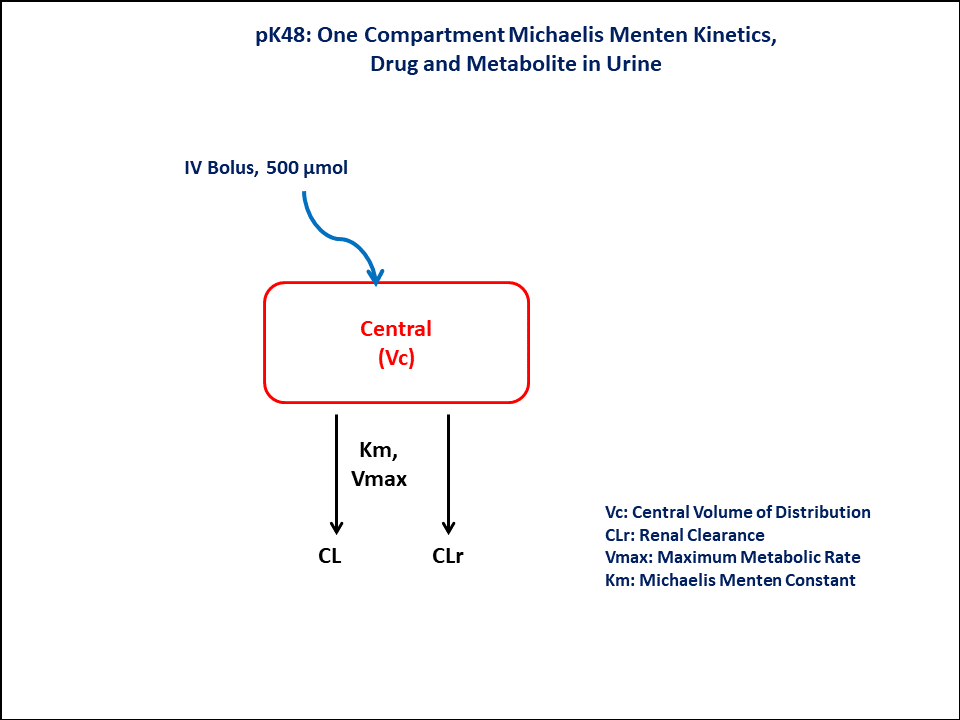
PK48 - One-compartment Michaelis-Menten kinetics - Drug and metabolite in urine

1 Background

Structural model - One Compartment Michaelis Menten Kinetics, Drug and metabolite in Urine
Route of administration - IV bolus
Dosage Regimen - 500 μmol IV
Number of Subjects - 1

2 Learning Outcome

In this model, you will learn

To build a one compartment model for the drug given Intravenous Bolus dosage, following Michaelis Menten Kinetics.
To apply differential equations in the model as per the compartment model.

3 Objectives

In this tutorial, you will learn how to build a one compartment Michaelis Menten Kinetics model, with drug and metabolite in urine.

4 Libraries

Call the necessary libraries to get started

using Random
using Pumas
using PumasUtilities
using CairoMakie
using AlgebraOfGraphics
using DataFramesMeta
using CSV
using Dates

5 Model

In this one compartment model, we administer the dose on the Central compartment.

pk_48 = @model begin
    @metadata begin
        desc = "One Compartment Michaelis Menten Kinetics Model"
        timeu = u"hr"
    end

    @param begin
        """
        Maximum rate of metabolism (μM/hr)
        """
        tvvmax ∈ RealDomain(lower = 0)
        """
        Michaelis Menten Constant (μM)
        """
        tvkm ∈ RealDomain(lower = 0)
        """
        Renal Clearance (L/hr)
        """
        tvclr ∈ RealDomain(lower = 0)
        """
        Central Volume of Distribution (L)
        """
        tvvc ∈ RealDomain(lower = 0)
        Ω ∈ PDiagDomain(4)
        """
        Proportional RUV
        """
        σ²_prop ∈ RealDomain(lower = 0)
    end

    @random begin
        η ~ MvNormal(Ω)
    end

    @pre begin
        Vmax = tvvmax * exp(η[1])
        Km = tvkm * exp(η[2])
        Clr = tvclr * exp(η[3])
        Vc = tvvc * exp(η[4])
    end

    @vars begin
        VMKM := Vmax * (Central / Vc) / (Km + (Central / Vc))
    end

    @dynamics begin
        Central' = -VMKM - (Clr / Vc) * Central
        UrineP' = (Clr / Vc) * Central
        UrineM' = VMKM
    end

    @derived begin
        cp = @. Central / Vc
        ae_p = @. UrineP
        ae_m = @. UrineM
        """
        Observed Concentration (μmol/L)
        """
        dv ~ @. Normal(cp, sqrt(cp^2 * σ²_prop))
        """
        Observed Amount (μmol)
        """
        dv_aep ~ @. Normal(ae_p, sqrt(cp^2 * σ²_prop))
        """
        Observed Amount (μmol)
        """
        dv_aem ~ @. Normal(ae_m, sqrt(cp^2 * σ²_prop))
    end
end

PumasModel
  Parameters: tvvmax, tvkm, tvclr, tvvc, Ω, σ²_prop
  Random effects: η
  Covariates:
  Dynamical system variables: Central, UrineP, UrineM
  Dynamical system type: Nonlinear ODE
  Derived: cp, ae_p, ae_m, dv, dv_aep, dv_aem
  Observed: cp, ae_p, ae_m, dv, dv_aep, dv_aem

6 Parameters

The parameters are as given below. Note that tv represents the typical value for parameters.

Vmax - Maximum rate of metabolism (μM/hr)
Km - Michaelis Menten Constant (μM)
Clr - Renal Clearance (L/hr)
Vc - Central Volume of Distribution (L)
Ω - Between Subject Variability
σ - Residual error

param = (;
    tvvmax = 51.4061,
    tvkm = 5.30997,
    tvclr = 2.46764,
    tvvc = 24.5279,
    Ω = Diagonal([0.04, 0.04, 0.04, 0.04]),
    σ²_prop = 0.02,
)

7 Dosage Regimen

Intravenous bolus dosing of 500 μmol to a single subject at time=0.

ev1 = DosageRegimen(500, cmt = 1, time = 0)

1×10 DataFrame

Row	time	cmt	amt	evid	ii	addl	rate	duration	ss	route
	Float64	Int64	Float64	Int8	Float64	Int64	Float64	Float64	Int8	NCA.Route
1	0.0	1	500.0	1	0.0	0	0.0	0.0	0	NullRoute

sub1 = Subject(id = 1, events = ev1)

Subject
  ID: 1
  Events: 1

8 Simulation

Let’s simulate for plasma concentration with the specific observation time points after the IV bolus dose. Since we are simulating only a single subject, we can zero out the random effects

zfx = zero_randeffs(pk_48, sub1, param)

(η = [0.0, 0.0, 0.0, 0.0],)

Random.seed!(123)

sim_sub1 = simobs(pk_48, sub1, param, zfx, obstimes = 0.1:0.1:15)

SimulatedObservations
  Simulated variables: cp, ae_p, ae_m, dv, dv_aep, dv_aem
  Time: 0.1:0.1:15.0

9 Visualization

df = @chain DataFrame(sim_sub1) begin
    dropmissing!(:cp)
    @rsubset :time ∈ [0, 1, 2, 3, 4, 5, 6, 7, 8, 10, 12, 14, 15]
    stack([:cp, :ae_p, :ae_m])
end

plt =
    data(df) *
    mapping(
        :time => "Time (hrs)",
        :value,
        color = :variable =>
            renamer([
                "cp" => "Parent Plasma Concentration",
                "ae_p" => "Parent Urine Amount",
                "ae_m" => "Metabolite Urine Amount",
            ]) => "Variable",
    ) *
    visual(ScatterLines; linewidth = 4, markersize = 12)
fig = Figure()
gridpos = fig[1, 1]

f = draw!(
    gridpos,
    plt,
    axis = (;
        yscale = log10,
        ytickformat = i -> (@. string(round(i; digits = 1))),
        xticks = 0:2:16,
        ylabel = "PK48 Concentrations (μmol/L) & Amount (μmol)",
    ),
)
legend!(
    gridpos,
    f;
    tellwidth = false,
    halign = :right,
    valign = :center,
    margin = (10, 10, 10, 10),
)
fig

10 Population simulation

par = (;
    tvvmax = 51.4061,
    tvkm = 5.30997,
    tvclr = 2.46764,
    tvvc = 24.5279,
    Ω = Diagonal([0.0432, 0.0368, 0.0213, 0.0123]),
    σ²_prop = 0.00140536,
)

ev1 = DosageRegimen(500, cmt = 1, time = 0)
pop = map(i -> Subject(id = i, events = ev1), 1:55)

Random.seed!(1234)
pop_sim = simobs(pk_48, pop, par, obstimes = [0, 1, 2, 3, 4, 5, 6, 7, 8, 10, 12, 14, 15])
sim_plot(pop_sim)

df_sim = DataFrame(pop_sim)

#CSV.write("pk_48.csv", df_sim)