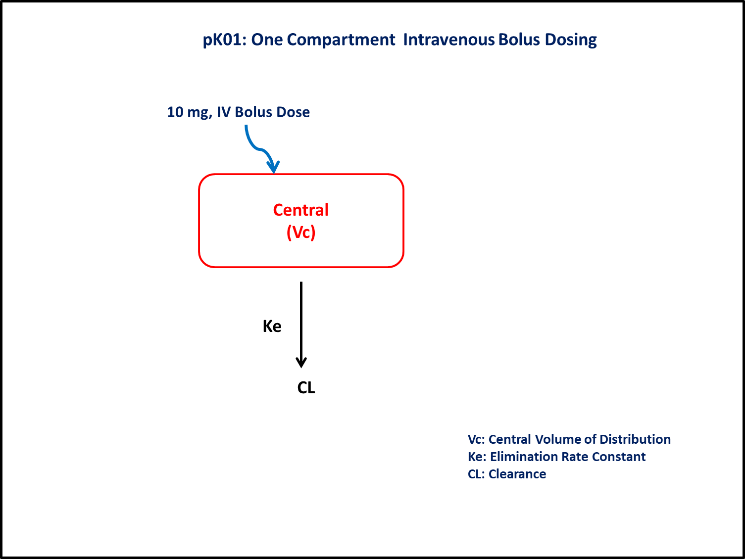
PK01 - One-compartment intravenous bolus dosing

1 Learning Outcome

Before constructing a model, it is important to establish the process the model will be following and a scenario for the simulation.

Below is the scenario for this tutorial:

To build a one compartment model for four subjects given Intravenous bolus dosage.
To estimate the fundamental parameters involved in building the model.
To apply differential equation in the model as per the compartment model.
To design the dosage regimen for the subjects and simulate the plot.

2 Objectives

In this tutorial, you will learn how to build a one compartment model and to simulate the model for four subjects with different disposition parameter estimates.

3 Background

Structural model - One compartment linear elimination
Route of administration - IV bolus
Dosage Regimen - 10 mg IV
Number of Subjects - 4

4 Libraries

Load the “necessary” libraries to get started.

using Pumas
using PumasUtilities
using Random
using AlgebraOfGraphics
using CairoMakie
using CSV
using DataFramesMeta
using Dates

5 Model

In this one compartment model, intravenous dose is administered into the central compartment.

Note

We account for rate of change of concentration of drug in plasma (Central Compartment) for the time duration up to 150 min.

pk_01 = @model begin
    @metadata begin
        desc = "One Compartment Model"
        timeu = u"minute"
    end
    @param begin
        """
        Clearance (L/hr)
        """
        tvcl ∈ RealDomain(lower = 0)
        """
        Volume (L)
        """
        tvvc ∈ RealDomain(lower = 0)
        """
        Additive RUV
        """
        σ ∈ RealDomain(lower = 0)
    end

    @pre begin
        Cl = tvcl
        Vc = tvvc
    end

    @dynamics begin
        Central' = -(Cl / Vc) * Central
    end

    @derived begin
        """
        PK01 Concentrations (μg/L)
        """
        cp = @. 1000 * (Central / Vc)
        """
        PK01 Concentrations (μg/L)
        """
        dv ~ @. Normal(cp, σ)
    end
end

PumasModel
  Parameters: tvcl, tvvc, σ
  Random effects:
  Covariates:
  Dynamical system variables: Central
  Dynamical system type: Matrix exponential
  Derived: cp, dv
  Observed: cp, dv

6 Parameters

In this exercise, parameter estimate values for each subject are different. For each subject, parameters are defined individually, wherein tv represents the typical value for parameters. Parameters provided for simulation are:

Cl - Clearance (L/hr)
Vc - Volume of Central Compartment (L)
Ω - Between Subject Variability
σ - Residual error

param_vec = [
    (tvcl = 0.10, tvvc = 9.98, σ = 15.80),
    (tvcl = 0.20, tvvc = 9.82, σ = 27.46),
    (tvcl = 0.20, tvvc = 10.22, σ = 8.78),
    (tvcl = 0.20, tvvc = 19.95, σ = 8.50),
]

7 Dosage Regimen

To start the simulation process, the dosing regimen specified in the background section must be developed first prior to running a simulation.

The DosageRegimen is specified as 10 mg IV bolus dosage administered to four subjects at time zero.

Note

The concentrations are in μg/L and dose is in mg, thus the final concentration is multiplied by 1000 in the model

ev1 = DosageRegimen(10; time = 0, cmt = 1)

1×10 DataFrame

Row	time	cmt	amt	evid	ii	addl	rate	duration	ss	route
	Float64	Int64	Float64	Int8	Float64	Int64	Float64	Float64	Int8	NCA.Route
1	0.0	1	10.0	1	0.0	0	0.0	0.0	0	NullRoute

This is how to create the population undergoing the dosing regimen above.

ids = [
    "1: CL = 0.10, V = 9.98",
    "2: CL = 0.20, V = 9.82",
    "3: CL = 0.20, V = 10.22",
    "4: CL = 0.20, V = 19.95",
]

pop = map(i -> Subject(; id = ids[i], events = ev1), 1:length(ids))

Population
  Subjects: 4
  Observations:

8 Simulation

Let’s simulate for plasma concentration for four subjects for specific observation time points after IV bolus dose.

Initialize the random number generator with a seed for reproducibility of the simulation.

Random.seed!(123)

Note

The Random.seed! function is included here for purposes of tutorial reproducibility and is not required in the Pumas workflow.

Define the time points at which concentration values will be simulated.

time_points = [10, 20, 30, 40, 50, 60, 70, 90, 110, 150]

sim = map(zip(pop, param_vec)) do (subj, p)
    return simobs(pk_01, subj, p, obstimes = time_points)
end

Simulated population (Vector{<:Subject})
  Simulated subjects: 4
  Simulated variables: cp, dv

9 Visualize results

@chain DataFrame(sim) begin
    dropmissing(:cp)
    data(_) *
    mapping(
        :time => "Time (hours)",
        :cp => "PK01 Concentration (μg/L)",
        color = :id => "",
    ) *
    visual(Lines, linewidth = 4)
    draw(;
        axis = (; xticks = time_points,),
        figure = (; fontsize = 22),
        legend = (position = :bottom, nbanks = 2, tellwidth = true),
    )
end