PK03 - One-compartment 1st and 0-order input

1 Objectives

In this tutorial, we will be looking at building a one compartment model for zero-order input and simulating the model for 1 subject.

2 Background

• Structural model - One compartment linear elimination with zero-order absorption
• Route of administration - Oral
• Dosage Regimen - 20 mg Oral
• Number of Subjects - 1

PK03 Graphic Model

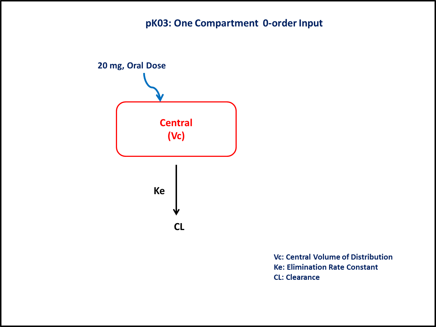
In this model, a collection of plasma concentration data will help us to derive/estimate the following parameters: Clearance, Volume of Distribution, and Duration of zero-order input.

3 Libraries

Call the required libraries to get started.

using Pumas
using PumasUtilities
using Random
using AlgebraOfGraphics
using CairoMakie
using CSV
using DataFramesMeta

4 Model

In this one compartment model, we administer the dose in the Central compartment as a zero-order input and estimate the rate of input.

pk_03 = @model begin
    @metadata begin
        desc = "One Compartment Model with zero-order input"
        timeu = u"hr"
    end

    @param begin
        """
        Clearance (L/hr)
        """
        tvcl ∈ RealDomain(lower = 0)
        """
        Volume (L)
        """
        tvvc ∈ RealDomain(lower = 0)
        """
        Assumed Duration of Zero-order (hr)
        """
        tvTabs ∈ RealDomain(lower = 0)
        Ω ∈ PDiagDomain(3)
        """
        Proportional RUV
        """
        σ²_prop ∈ RealDomain(lower = 0)
    end

    @random begin
        η ~ MvNormal(Ω)
    end

    @pre begin
        Cl = tvcl * exp(η[1])
        Vc = tvvc * exp(η[2])
    end

    @dosecontrol begin
        duration = (Central = tvTabs * exp(η[3]),)
    end

    @dynamics begin
        Central' = -(Cl / Vc) * Central
    end

    @derived begin
        """
        PK03 Concentration (μg/L)
        """
        cp = @. 1000 * (Central / Vc)
        """
        PK03 Concentration (μg/L)
        """
        dv ~ @. Normal(cp, sqrt(cp^2 * σ²_prop))
    end
end

PumasModel
  Parameters: tvcl, tvvc, tvTabs, Ω, σ²_prop
  Random effects: η
  Covariates: 
  Dynamical system variables: Central
  Dynamical system type: Matrix exponential
  Derived: cp, dv
  Observed: cp, dv

5 Parameters

Parameters provided for simulation:

• Cl - Clearance (L/hr)
• Vc - Volume of Central Compartment (L)
• Tabs - Assumed duration of zero-order input (hrs)
• Ω - Between Subject Variability
• σ - Residual error

These are the initial estimates we will be using in this model exercise. tv represents the typical value for parameters.

param_03 = (;
    tvcl = 45.12,
    tvvc = 96,
    tvTabs = 4.54,
    Ω = Diagonal([0.08, 0.03, 0.0226]),
    σ²_prop = 0.015,
)

6 Dosage Regimen

Single 20 mg or 20000 μg oral dose given to a subject.

Note

In this the dose administered is on mg and conc are in μg/L, hence a scaling factor of 1000 is used in the @derived block in the model.

ev1 = DosageRegimen(20; rate = -2)

1×10 DataFrame

Row	time	cmt	amt	evid	ii	addl	rate	duration	ss	route
	Float64	Int64	Float64	Int8	Float64	Int64	Float64	Float64	Int8	NCA.Route
1	0.0	1	20.0	1	0.0	0	-2.0	0.0	0	NullRoute

sub = Subject(; id = 1, events = ev1, observations = (cp = nothing,))

Subject
  ID: 1
  Events: 2
  Observations: cp: (n=0)

7 Simulation

Let’s simulate for plasma concentration with the specific observation time points after oral administration.

Note

The Random.seed! function is included here for purposes of reproducibility of the simulation in this tutorial. Specification of a seed value would not be required in a Pumas workflow that is estimating model parameters.

Random.seed!(123)

The random effects are zero’ed out since we are simulating means

zfx = zero_randeffs(pk_03, sub, param_03)

sim = simobs(pk_03, sub, param_03, zfx, obstimes = 0:0.1:10)

SimulatedObservations
  Simulated variables: cp, dv
  Time: 0.0:0.1:10.0

8 Visualize results

@chain DataFrame(sim) begin
    dropmissing(:cp)
    data(_) *
    mapping(:time => "Time (hours)", :cp => "PK03 Concentration (μg/L)") *
    visual(Lines, linewidth = 4)
    draw(; axis = (; xticks = 0:1:10,), figure = (; fontsize = 22))
end

9 Population Simulation

This block updates the parameters of the model to increase intersubject variability in parameters and defines time points for the prediction of concentrations. The results are written to a CSV file.

par = (
    tvcl = 45.12,
    tvvc = 96,
    tvTabs = 4.54,
    Ω = Diagonal([0.09, 0.04, 0.0225]),
    σ²_prop = 0.015,
)

ev1 = DosageRegimen(20; rate = -2)
pop = map(i -> Subject(id = i, events = ev1), 1:90)

Random.seed!(1234)
sim_pop = simobs(pk_03, pop, par, obstimes = [0, 0.5, 1, 1.5, 2, 3, 4, 5, 6, 7, 8, 9, 10])

df_sim = DataFrame(sim_pop);

#CSV.write("pk_03.csv", df_sim)