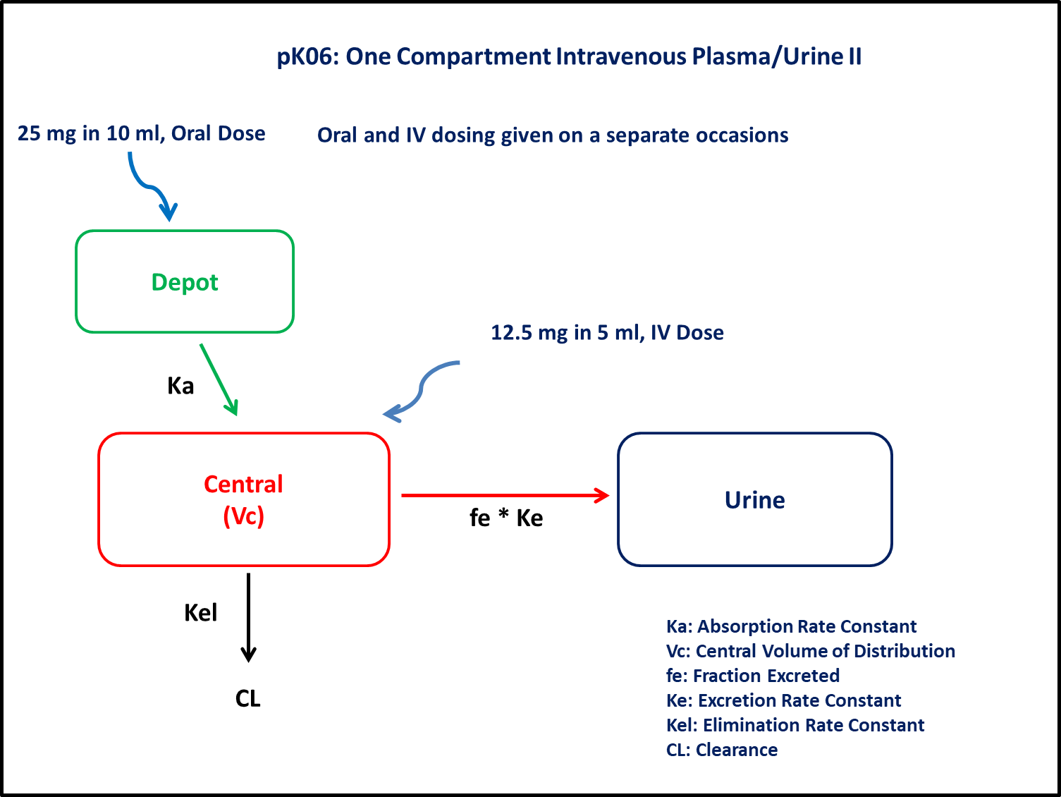
PK06 - One-compartment intravenous plasma/urine II

1 Background

Structural model - One compartment linear elimination with first order absorption
Route of administration - Oral and IV given simultaneously
Dosage Regimen - 12.5 mg IV and 25 mg Oral
Number of Subjects - 1

2 Objective

In this tutorial, you will learn to build a one compartment model and to simulate the model for different subjects and dosage regimens.

3 Libraries

Call the necessary libraries to get started

using Pumas
using PumasUtilities
using AlgebraOfGraphics
using CairoMakie
using ColorSchemes
using Random
using CSV
using DataFramesMeta
using Dates

4 Model

In this one compartment model, we administer doses both oral and IV on two different occasions.

pk_06 = @model begin
    @metadata begin
        desc = "One Compartment Model with Urine Cmt"
        timeu = u"hr"
    end

    @param begin
        """
        Clearance (L/hr)
        """
        tvcl ∈ RealDomain(lower = 0)
        """
        Volume of Distribution (L)
        """
        tvvc ∈ RealDomain(lower = 0)
        """
        Fraction of drug excreted in Urine
        """
        tvfe ∈ RealDomain(lower = 0)
        """
        Absorption Rate Constant (1/hr)
        """
        tvka ∈ RealDomain(lower = 0)
        """
        Lag-time (hr)
        """
        tvlag ∈ RealDomain(lower = 0)
        """
        Bioavailability
        """
        tvF ∈ RealDomain(lower = 0)
        Ω ∈ PDiagDomain(6)
        """
        Proportional RUV
        """
        σ²_prop ∈ RealDomain(lower = 0)
        """
        Additive RUV
        """
        σ_add ∈ RealDomain(lower = 0)
    end

    @random begin
        η ~ MvNormal(Ω)
    end

    @pre begin
        Cl = tvcl * exp(η[1])
        Vc = tvvc * exp(η[2])
        Ka = tvka * exp(η[3])
        fe = tvfe * exp(η[4])
    end

    @dosecontrol begin
        lags = (Depot = tvlag * exp(η[5]),)
        bioav = (Depot = tvF * exp(η[6]),)
    end

    @dynamics begin
        Depot' = -Ka * Depot
        Central' = Ka * Depot - (Cl / Vc) * Central
        Urine' = fe * (Cl / Vc) * Central
    end

    @derived begin
        """
        PK06 Plasma Concentration (μg/L)
        """
        cp = @. (Central / Vc)
        dv ~ @. Normal(cp, sqrt(cp^2 * σ²_prop))

        """
        PK06 Urine Amount (μg)
        """
        ae = @. Urine
        dv_ae ~ @. Normal(ae, σ_add)
    end
end

PumasModel
  Parameters: tvcl, tvvc, tvfe, tvka, tvlag, tvF, Ω, σ²_prop, σ_add
  Random effects: η
  Covariates:
  Dynamical system variables: Depot, Central, Urine
  Dynamical system type: Nonlinear ODE
  Derived: cp, dv, ae, dv_ae
  Observed: cp, dv, ae, dv_ae

5 Parameters

Parameters provided for simulation. Note that tv represents the typical value for parameters.

Cl - Clearance (L/hr)
Vc - Volume of Central Compartment (L)
Fe - Fraction of drug excreted in Urine
lag - lag time (hr)
Ka - Absorption rate constant (hr⁻¹)
F - Bioavailability
Ω - Between Subject Variability
σ - Residual error

param = (
    tvcl = 6.02527,
    tvvc = 290.292,
    tvfe = 0.0698294,
    tvka = 0.420432,
    tvlag = 0.311831,
    tvF = 1.13591,
    Ω = Diagonal([0.04, 0.04, 0.04, 0.04, 0.04, 0.04]),
    σ²_prop = 0.015,
    σ_add = 3,
)

6 Dosage Regimen

6.1 For IV

A single subject receives an IV-bolus dose of 12.5 mg or 12500 μg

ev1 = DosageRegimen(12500, time = 0, cmt = 2)

1×10 DataFrame

Row	time	cmt	amt	evid	ii	addl	rate	duration	ss	route
	Float64	Int64	Float64	Int8	Float64	Int64	Float64	Float64	Int8	NCA.Route
1	0.0	2	12500.0	1	0.0	0	0.0	0.0	0	NullRoute

sub1 = Subject(id = "1 - IV", events = ev1)

Subject
  ID: 1 - IV
  Events: 1

6.2 For Oral

A single subject receives an oral dose of 25 mg or 25000 μg

ev2 = DosageRegimen(25000, time = 0, cmt = 1)

1×10 DataFrame

Row	time	cmt	amt	evid	ii	addl	rate	duration	ss	route
	Float64	Int64	Float64	Int8	Float64	Int64	Float64	Float64	Int8	NCA.Route
1	0.0	1	25000.0	1	0.0	0	0.0	0.0	0	NullRoute

sub2 = Subject(id = "2 - PO", events = ev2)

Subject
  ID: 2 - PO
  Events: 1

pop = [sub1, sub2]

Population
  Subjects: 2
  Observations:

7 Simulation

Here, we will learn how to simultaneously simulate plasma concentration and urine amount after IV and oral administration.

Random.seed!(123)

The random effects are zero’ed out since we are simulating means

zfx = zero_randeffs(pk_06, pop, param)

2-element Vector{@NamedTuple{η::Vector{Float64}}}:
 (η = [0.0, 0.0, 0.0, 0.0, 0.0, 0.0],)
 (η = [0.0, 0.0, 0.0, 0.0, 0.0, 0.0],)

sim = simobs(pk_06, pop, param, zfx, obstimes = 0.1:0.1:168)

Simulated population (Vector{<:Subject})
  Simulated subjects: 2
  Simulated variables: cp, dv, ae, dv_ae

7.1 For IV

Let’s simulate for plasma concentration and amount excreted unchanged in urine.

The random effects are zero’ed out since we are simulating means

zfx = zero_randeffs(pk_06, sub1, param)

(η = [0.0, 0.0, 0.0, 0.0, 0.0, 0.0],)

sim_sub1_iv = simobs(pk_06, sub1, param, zfx, obstimes = 0.1:0.1:168)

SimulatedObservations
  Simulated variables: cp, dv, ae, dv_ae
  Time: 0.1:0.1:168.0

df_sim_iv = DataFrame(sim_sub1_iv)
first(df_sim_iv, 5)

5×31 DataFrame

Row	id	time	cp	dv	ae	dv_ae	evid	lags_Depot	bioav_Depot	amt	cmt	rate	duration	ss	ii	route	tad	dosenum	Depot	Central	Urine	Cl	Vc	Ka	fe	η_1	η_2	η_3	η_4	η_5	η_6
	String	Float64	Float64?	Float64?	Float64?	Float64?	Int64	Float64?	Float64?	Float64?	Symbol?	Float64?	Float64?	Int8?	Float64?	NCA.Route?	Float64	Int64	Float64?	Float64?	Float64?	Float64?	Float64?	Float64?	Float64?	Float64	Float64	Float64	Float64	Float64	Float64
1	1 - IV	0.0	missing	missing	missing	missing	1	0.311831	1.13591	12500.0	Central	0.0	0.0	0	0.0	NullRoute	0.0	1	missing	missing	missing	6.02527	290.292	0.420432	0.0698294	0.0	0.0	0.0	0.0	0.0	0.0
2	1 - IV	0.1	42.9708	34.4261	1.80984	1.15684	0	missing	missing	0.0	missing	0.0	0.0	0	0.0	missing	0.1	1	0.0	12474.1	1.80984	6.02527	290.292	0.420432	0.0698294	0.0	0.0	0.0	0.0	0.0	0.0
3	1 - IV	0.2	42.8817	45.4669	3.61592	6.55886	0	missing	missing	0.0	missing	0.0	0.0	0	0.0	missing	0.2	1	0.0	12448.2	3.61592	6.02527	290.292	0.420432	0.0698294	0.0	0.0	0.0	0.0	0.0	0.0
4	1 - IV	0.3	42.7928	43.2119	5.41826	10.0656	0	missing	missing	0.0	missing	0.0	0.0	0	0.0	missing	0.3	1	0.0	12422.4	5.41826	6.02527	290.292	0.420432	0.0698294	0.0	0.0	0.0	0.0	0.0	0.0
5	1 - IV	0.4	42.7041	35.6872	7.21686	8.45334	0	missing	missing	0.0	missing	0.0	0.0	0	0.0	missing	0.4	1	0.0	12396.7	7.21686	6.02527	290.292	0.420432	0.0698294	0.0	0.0	0.0	0.0	0.0	0.0

7.2 For Oral

Let’s simulate the plasma concentration and amount excreted unchanged in urine.

The random effects are zero’ed out since we are simulating means

zfx = zero_randeffs(pk_06, sub2, param)

(η = [0.0, 0.0, 0.0, 0.0, 0.0, 0.0],)

sim_sub2_oral = simobs(pk_06, sub2, param, obstimes = 0.1:0.1:168)

SimulatedObservations
  Simulated variables: cp, dv, ae, dv_ae
  Time: 0.1:0.1:168.0

df_sim_oral = DataFrame(sim_sub2_oral)
first(df_sim_oral, 5)

5×31 DataFrame

Row	id	time	cp	dv	ae	dv_ae	evid	lags_Depot	bioav_Depot	amt	cmt	rate	duration	ss	ii	route	tad	dosenum	Depot	Central	Urine	Cl	Vc	Ka	fe	η_1	η_2	η_3	η_4	η_5	η_6
	String	Float64	Float64?	Float64?	Float64?	Float64?	Int64	Float64?	Float64?	Float64?	Symbol?	Float64?	Float64?	Int8?	Float64?	NCA.Route?	Float64	Int64	Float64?	Float64?	Float64?	Float64?	Float64?	Float64?	Float64?	Float64	Float64	Float64	Float64	Float64	Float64
1	2 - PO	0.0	missing	missing	missing	missing	1	0.281472	0.999388	25000.0	Depot	0.0	0.0	0	0.0	NullRoute	0.0	1	missing	missing	missing	5.71161	264.931	0.325862	0.0585771	-0.0534609	-0.0914181	-0.254808	-0.175711	-0.102428	-0.128046
2	2 - PO	0.1	0.0	0.0	0.0	0.116066	0	missing	missing	0.0	missing	0.0	0.0	0	0.0	missing	0.1	1	0.0	0.0	0.0	5.71161	264.931	0.325862	0.0585771	-0.0534609	-0.0914181	-0.254808	-0.175711	-0.102428	-0.128046
3	2 - PO	0.2	0.0	0.0	0.0	5.03178	0	missing	missing	0.0	missing	0.0	0.0	0	0.0	missing	0.2	1	0.0	0.0	0.0	5.71161	264.931	0.325862	0.0585771	-0.0534609	-0.0914181	-0.254808	-0.175711	-0.102428	-0.128046
4	2 - PO	0.3	0.567549	0.58451	0.00176097	-2.27266	0	missing	missing	0.0	missing	0.0	0.0	0	0.0	missing	0.3	1	24834.3	150.361	0.00176097	5.71161	264.931	0.325862	0.0585771	-0.0534609	-0.0914181	-0.254808	-0.175711	-0.102428	-0.128046
5	2 - PO	0.4	3.56843	3.42717	0.0712408	-1.93059	0	missing	missing	0.0	missing	0.0	0.0	0	0.0	missing	0.4	1	24038.1	945.388	0.0712408	5.71161	264.931	0.325862	0.0585771	-0.0534609	-0.0914181	-0.254808	-0.175711	-0.102428	-0.128046

@rsubset! df_sim_oral :time > 0.2

8 Visualization

Combined Plot of IV data and Oral data

plasma_times = [0.3, 0.6, 1, 2, 3, 4, 6, 8, 24, 48, 72, 96, 168]
df_iv_plasma = @rsubset df_sim_iv :time in plasma_times
df_oral_plasma = @rsubset df_sim_oral :time in plasma_times

urine_times = [24, 48]
df_iv_urine = @rsubset df_sim_iv :time in urine_times
df_oral_urine = @rsubset df_sim_oral :time in urine_times

ivsim_plt = @chain df_sim_iv begin
    @rtransform :Type = "IV Prediction"
    dropmissing(:cp)
    data(_) *
    mapping(
        :time => "Time (hours)",
        :cp => "Concentration (μg/L) & Amount (μg)",
        color = :Type,
    ) *
    visual(Lines, linewidth = 4)
end

iv_plt = @chain df_iv_plasma begin
    @rtransform :Type = "IV Observations"
    dropmissing(:cp)
    data(_) *
    mapping(
        :time => "Time (hours)",
        :cp => "Concentration (μg/L) & Amount (μg)",
        color = :Type,
    ) *
    visual(Scatter, color = :blue, markersize = 14)
end

ivurine_plt = @chain df_iv_urine begin
    @rtransform :Type = "IV Observations Amount"
    dropmissing(:ae)
    data(_) *
    mapping(
        :time => "Time (hours)",
        :ae => "Concentration (μg/L) & Amount (μg)",
        color = :Type,
    ) *
    visual(ScatterLines, color = :blue, markersize = 14, linewidth = 4)
end

oralsim_plt = @chain df_sim_oral begin
    @rtransform :Type = "Oral Prediction"
    dropmissing(:cp)
    data(_) *
    mapping(
        :time => "Time (hours)",
        :cp => "Concentration (μg/L) & Amount (μg)",
        color = :Type,
    ) *
    visual(Lines, linewidth = 4)
end

oral_plt = @chain df_oral_plasma begin
    @rtransform :Type = "Oral Observations"
    dropmissing(:cp)
    data(_) *
    mapping(
        :time => "Time (hours)",
        :cp => "Concentration (μg/L) & Amount (μg)",
        color = :Type,
    ) *
    visual(Scatter, markersize = 14)
end

oralurine_plt = @chain df_oral_urine begin
    @rtransform :Type = "Oral Observations Amount"
    dropmissing(:ae)
    data(_) *
    mapping(
        :time => "Time (hours)",
        :ae => "Concentration (μg/L) & Amount (μg)",
        color = :Type,
    ) *
    visual(ScatterLines, markersize = 14, linewidth = 4)
end

draw(
    ivsim_plt + iv_plt + ivurine_plt + oralsim_plt + oral_plt + oralurine_plt,
    scales(Color = (; palette = :tableau_10));
    axis = (;
        xticks = [0, 20, 40, 60, 80, 100, 120, 140, 160, 180],
        yscale = Makie.Symlog10(10),
        yticks = [1, 10, 100, 1000, 2000],
        ytickformat = x -> string.(round.(x; digits = 1)),
        ygridwidth = 3,
        yminorticksvisible = true,
        yminorgridvisible = true,
        yminorticks = IntervalsBetween(10),
        xminorticksvisible = true,
        xminorgridvisible = true,
        xminorticks = IntervalsBetween(5),
    ),
    figure = (; fontsize = 22),
    legend = (position = :bottom, nbanks = 3, tellwidth = true),
)