using Random
using Pumas
using PumasUtilities
using AlgebraOfGraphics
using CairoMakie
using CSV
using DataFramesMeta
using Dates
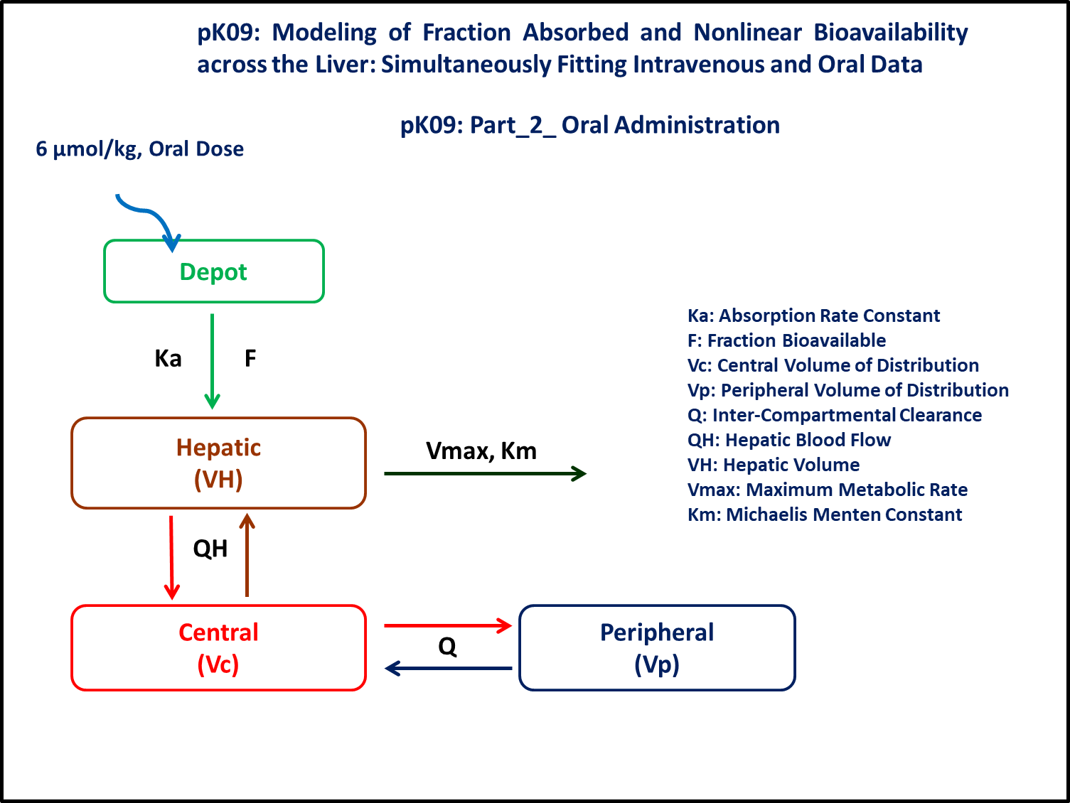
PK09 - Modeling of fraction absorbed and nonlinear bioavailability across the liver
1 Background
- Structural model - Two compartment model with non-linear elimination from the hepatic compartment
- Route of administration - Oral and IV on separate occasions
- Dosage Regimen - 2 μmol/kg IV and 6 μmol/kg Oral
- Number of Subjects - 1
2 Learning Outcomes
Semi-physiologic model with elimination from the hepatic compartment and dose administered by IV bolus. The drug follows a two compartment model. This data was modeled taking into account the hepatic elimination component and hepatic blood flow. Hepatic distribution and elimination from the liver is modeled as an additional compartment with physiological values of blood flow reported from the literature. Oral doses are administered into a Depot. This Depot compartment was connected to the liver compartment. This study was conducted with an Oral suspension of 6 μmol/kg and an IV bolus of 2 μmol/kg.
3 Objective
The exercise aims to simulate data using a two compartment model and an additional hepatic compartment. The elimination is non-linear metabolic clearance from the liver. In the case of oral administration, the administered dose reaches the hepatic compartment with a lag-time.
4 Libraries
Call the necessary libraries to get started
5 Model
This model is written for both oral and IV dosing regimen
pk_09 = @model begin
    @metadata begin
        desc = "Semi-Physiologic Model"
        timeu = u"hr"
    end

    @param begin
        """
        Volume of Central Compartment (L/kg)
        """
        tvvc ∈ RealDomain(lower = 0)
        """
        Inter-compartmental Clearance (L/hr/kg)
        """
        tvq ∈ RealDomain(lower = 0)
        """
        Volume of Peripheral Compartment (L/kg)
        """
        tvvp ∈ RealDomain(lower = 0)
        """
        Maximum Metabolic Rate (μmol/hr/kg)
        """
        tvvmax ∈ RealDomain(lower = 0)
        """
        Michaelis Menton Constant (μmol/L)
        """
        tvkm ∈ RealDomain(lower = 0)
        """
        Absorption Rate Constant (hr⁻¹)
        """
        tvka ∈ RealDomain(lower = 0)
        """
        Lag-time (hr)
        """
        tvtlag ∈ RealDomain(lower = 0)
        """
        Fraction of drug absorbed
        """
        tvfa ∈ RealDomain(lower = 0)
        Ω ∈ PDiagDomain(8)
        """
        Proportional RUV
        """
        σ²_prop ∈ RealDomain(lower = 0)
    end

    @random begin
        η ~ MvNormal(Ω)
    end

    @pre begin
        Vc = tvvc * exp(η[1])
        Q = tvq * exp(η[2])
        Vp = tvvp * exp(η[3])
        Vmax = tvvmax * exp(η[4])
        Km = tvkm * exp(η[5])
        Ka = tvka * exp(η[6])
        Qh = 3.3
        Vh = 0.02
    end

    @dosecontrol begin
        lags = (Depot = tvtlag * exp(η[7]),)
        bioav = (Depot = tvfa * exp(η[8]),)
    end

    @vars begin
        VMKM := Vmax * (Hepatic / Vh) / (Km + (Hepatic / Vh))
    end

    @dynamics begin
        Depot' = -Ka * Depot
        Hepatic' = Ka * Depot - (Qh / Vh) * Hepatic + (Qh / Vc) * Central - VMKM
        Central' =
            (Qh / Vh) * Hepatic - (Qh / Vc) * Central - (Q / Vc) * Central +
            (Q / Vp) * Peripheral
        Peripheral' = (Q / Vc) * Central - (Q / Vp) * Peripheral
    end

    @derived begin
        cp = @. Central / Vc
        """
        Observed Concentration (μg/L)
        """
        dv ~ ProportionalNormal.(cp, sqrt(σ²_prop))
    end
end
┌ Warning: Variable `cp` is defined in the `@derived` block using `=` and hence `cp` is not used for model fitting but only returned when simulating: │ If `cp` is a random variable, it must be defined in the `@derived` block using `~`; │ if `cp` should be returned when simulating, it should be defined in the `@observed` block using `=`; │ if `cp` is an intermediate quantity that should not be returned when simulating, it should be defined using `:=`. └ @ Pumas ~/run/_work/PumasTutorials.jl/PumasTutorials.jl/custom_julia_depot/packages/Pumas/GZeMg/src/dsl/model_macro.jl:2351
PumasModel
  Parameters: tvvc, tvq, tvvp, tvvmax, tvkm, tvka, tvtlag, tvfa, Ω, σ²_prop
  Random effects: η
  Covariates:
  Dynamical system variables: Depot, Hepatic, Central, Peripheral
  Dynamical system type: Nonlinear ODE
  Derived: cp, dv
  Observed: cp, dv
6 Parameters
Parameters provided for simulation. Note that tv represents the typical value for parameters.
Vc- Volume of Central Compartment (L/kg)Q- Intercompartmental Clearance (L/kg)Vp- Volume of Peripheral Compartment (L/kg)Vmax- Maximum Metabolic Rate (μmol/hr/kg)Km- Michaelis Menton Constant (μmol/L)Ka- Absorption Rate Constant (hr⁻¹)fa- Fraction of drug absorbedtlag- lag time (hr)
param = (
    tvvc = 0.34,
    tvq = 1.84,
    tvvp = 0.38,
    tvvmax = 0.13,
    tvkm = 0.31,
    tvka = 11.3,
    tvfa = 0.38,
    tvtlag = 0.062,
    Ω = Diagonal([0.04, 0.04, 0.04, 0.04, 0.04, 0.04, 0.04, 0.04]),
    σ²_prop = 0.001,
)
7 Dosage Regimen
7.1 Oral
Dose of 6 μmol/kg is administered orally at time=0
ev1 = DosageRegimen(6, time = 0, cmt = :Depot)1×10 DataFrame
| Row | time | cmt | amt | evid | ii | addl | rate | duration | ss | route |
|---|---|---|---|---|---|---|---|---|---|---|
| Float64 | Symbol | Float64 | Int8 | Float64 | Int64 | Float64 | Float64 | Int8 | NCA.Route | |
| 1 | 0.0 | Depot | 6.0 | 1 | 0.0 | 0 | 0.0 | 0.0 | 0 | NullRoute |
sub1 = Subject(id = "1: PO", events = ev1)Subject
ID: 1: PO
Events: 17.2 IV
Dose of 2 μmol/kg is administered as IV-bolus at time=0
ev2 = DosageRegimen(2, time = 0, cmt = :Central)1×10 DataFrame
| Row | time | cmt | amt | evid | ii | addl | rate | duration | ss | route |
|---|---|---|---|---|---|---|---|---|---|---|
| Float64 | Symbol | Float64 | Int8 | Float64 | Int64 | Float64 | Float64 | Int8 | NCA.Route | |
| 1 | 0.0 | Central | 2.0 | 1 | 0.0 | 0 | 0.0 | 0.0 | 0 | NullRoute |
sub2 = Subject(id = "2: IV", events = ev2)Subject
ID: 2: IV
Events: 18 Simulation
8.1 Oral
Random.seed!(123)The random effects are zero’ed out since we are simulating means
zfx = zero_randeffs(pk_09, sub1, param)(η = [0.0, 0.0, 0.0, 0.0, 0.0, 0.0, 0.0, 0.0],)sim_sub1_oral =
simobs(pk_09, sub1, param, zfx, obstimes = [0.08333, 0.25, 0.5, 1, 2, 4, 6, 8, 23])SimulatedObservations
Simulated variables: cp, dv
Time: [0.08333, 0.25, 0.5, 1.0, 2.0, 4.0, 6.0, 8.0, 23.0]8.2 IV
The random effects are zero’ed out since we are simulating means
zfx = zero_randeffs(pk_09, sub2, param)(η = [0.0, 0.0, 0.0, 0.0, 0.0, 0.0, 0.0, 0.0],)sim_sub2_iv = simobs(
pk_09,
sub2,
param,
zfx,
obstimes = [0.0056, 0.03333, 0.13333, 0.25, 0.75, 1, 2, 3, 4, 6, 8, 10, 12, 15, 20, 23],
)SimulatedObservations
Simulated variables: cp, dv
Time: [0.0056, 0.03333, 0.13333, 0.25, 0.75, 1.0, 2.0, 3.0, 4.0, 6.0, 8.0, 10.0, 12.0, 15.0, 20.0, 23.0]9 Visualization
po_plt = @chain DataFrame(sim_sub1_oral) begin
    @rtransform :Route = "Oral"
    dropmissing(:cp)
    data(_) *
    mapping(:time => "Time (hours)", :cp => "PK9 Concentration (μM)", color = :Route) *
    visual(ScatterLines, color = :blue, linewidth = 4)
end

iv_plt = @chain DataFrame(sim_sub2_iv) begin
    @rtransform :Route = "IV"
    dropmissing(:cp)
    data(_) *
    mapping(:time => "Time (hours)", :cp => "PK9 Concentration (μM)", color = :Route) *
    visual(ScatterLines, color = :black, linewidth = 4)
end

draw(
    po_plt + iv_plt;
    axis = (;
        xticks = 0:5:25,
        yticks = map(i -> 10^i, -1:0.5:1),
        yscale = log10,
        ytickformat = x -> string.(round.(x; digits = 1)),
        ygridwidth = 3,
        yminorticksvisible = true,
        yminorgridvisible = true,
        yminorticks = IntervalsBetween(20),
        xminorticksvisible = true,
        xminorgridvisible = true,
        xminorticks = IntervalsBetween(5),
    ),
    figure = (; fontsize = 22),
)
10 Population simulation
par = (
    tvvc = 0.34,
    tvq = 1.84,
    tvvp = 0.38,
    tvvmax = 0.13,
    tvkm = 0.31,
    tvka = 11.3,
    tvfa = 0.38,
    tvtlag = 0.062,
    Ω = Diagonal([0.0081, 0.044, 0.0081, 0.0121, 0.184, 0.0225, 0.0009, 0.0025]),
    σ²_prop = 0.0152,
)

## Oral
ev1 = DosageRegimen(6, time = 0, cmt = :Depot)
pop_oral = map(i -> Subject(id = i, events = ev1), 1:30)

Random.seed!(1234)
sim_pop_oral =
    simobs(pk_09, pop_oral, par, obstimes = [0.08333, 0.25, 0.5, 1, 2, 4, 6, 8, 23])

df_pop_oral = DataFrame(sim_pop_oral)
df_pop_oral[!, :route] .= "Oral"

## IV
ev2 = DosageRegimen(2, time = 0, cmt = :Central)
pop_iv = map(i -> Subject(id = i, events = ev2), 1:30)

Random.seed!(1234)
sim_pop_iv = simobs(
    pk_09,
    pop_iv,
    par,
    obstimes = [0.0056, 0.03333, 0.13333, 0.25, 0.75, 1, 2, 3, 4, 6, 8, 10, 12, 15, 20, 23],
)
sim_plot(sim_pop_iv)
df_pop_iv = DataFrame(sim_pop_iv)
df_pop_iv[!, :route] .= "IV"

df_sim = vcat(df_pop_oral, df_pop_iv);

#CSV.write("pk_09.csv", df_sim)