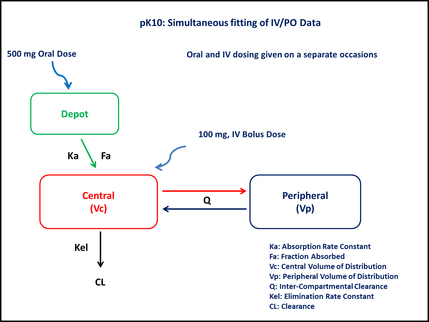
PK10 - Simultaneous fitting of IV/PO data

1 Background

• Structural model - Two compartment linear elimination with first order absorption
• Route of administration - IV bolus and oral given on separate occasions
• Dosage regimens - 100 mg IV Bolus and 500 mg Oral
• Subject - 1

PK10 Model Graphic

2 Learning Outcome

This exercise demonstrates simultaneous fitting of IV/PO data and will help you understand the disposition of drugs following IV and oral administration (with and without lag time).

3 Objectives

To build a two-compartment model, simulate the model for a single subject given IV bolus and oral dose on separate occasions and subsequently perform simulation for a population.

4 Libraries

Load the necessary libraries.

using PumasUtilities
using Random
using Pumas
using CairoMakie
using AlgebraOfGraphics
using CSV
using DataFramesMeta
using Dates

5 Model definition

Note the expression of the model parameters with helpful comments. The model is expressed with differential equations. Residual variability is a proportional error model.

In this two compartment model, we administer doses to the Depot and Central compartments.

pk_10 = @model begin
    @metadata begin
        desc = "Two Compartment Model"
        timeu = u"minute"
    end

    @param begin
        """
        Volume of Central Compartment (L)
        """
        tvvc ∈ RealDomain(lower = 0)
        """
        Volume of Peripheral Compartment (L)
        """
        tvvp ∈ RealDomain(lower = 0)
        """
        InterCompartmental Clearance (L/min)
        """
        tvq ∈ RealDomain(lower = 0)
        """
        Clearance (L/min)
        """
        tvcl ∈ RealDomain(lower = 0)
        """
        Absorption Rate Constant (min⁻¹)
        """
        tvka ∈ RealDomain(lower = 0)
        """
        Fraction of drug absorbed
        """
        tvfa ∈ RealDomain(lower = 0)
        """
        Lagtime (min)
        """
        tvlag ∈ RealDomain(lower = 0)
        Ω ∈ PDiagDomain(7)
        """
        Proportional RUV
        """
        σ²_prop ∈ RealDomain(lower = 0)
    end

    @random begin
        η ~ MvNormal(Ω)
    end

    @pre begin
        Vc = tvvc * exp(η[1])
        Vp = tvvp * exp(η[2])
        Q = tvq * exp(η[3])
        CL = tvcl * exp(η[4])
        Ka = tvka * exp(η[5])
    end

    @dosecontrol begin
        bioav = (Depot = tvfa * exp(η[6]),)
        lags = (Depot = tvlag * exp(η[7]),)
    end

    @dynamics Depots1Central1Periph1

    @derived begin
        cp = @. Central / Vc
        """
        Observed Concentration (mg/L)
        """
        dv ~ @. Normal(cp, sqrt(cp^2 * σ²_prop))
    end
end

PumasModel
  Parameters: tvvc, tvvp, tvq, tvcl, tvka, tvfa, tvlag, Ω, σ²_prop
  Random effects: η
  Covariates: 
  Dynamical system variables: Depot, Central, Peripheral
  Dynamical system type: Closed form
  Derived: cp, dv
  Observed: cp, dv

6 Initial Estimates of Model Parameters

The model parameters for simulation are the following. Note that tv represents the typical value for parameters.

• Vc - Volume of Central Compartment (L)
• Vp - Volume of Peripheral Compartment (L)
• Q - InterCompartmental clearance (L/min)
• Cl - Clearance from Central InterCompartmental (L/min)
• Ka - Absorption rate constant (min⁻¹)
• Fa - Fraction of drug absorbed
• lags - Lagtime (min)
• Ω - Between Subject Variability
• σ - Residual error

6.1 IV / PO - without lagtime

A vector of model parameter values is defined.

param1 = (
    tvvc = 59.9348,
    tvvp = 60.5898,
    tvq = 1.55421,
    tvcl = 0.967573,
    tvka = 0.0471557,
    tvfa = 0.318748,
    tvlag = 14.8187,
    Ω = Diagonal([0.01, 0.01, 0.01, 0.01, 0.01, 0.01, 0.01]),
    σ²_prop = 0.01,
)

6.2 IV / PO - with lagtime

param2 = (param1..., tvlag = 14.8187)

7 Dosage Regimen and Subjects

Dosage Regimen - single subject receiving 100 mg Intravenous bolus dose and 500 mg oral dose on different occasions.

7.1 IV

ev1 = DosageRegimen(100, time = 0, cmt = 2)

1×10 DataFrame

Row	time	cmt	amt	evid	ii	addl	rate	duration	ss	route
	Float64	Int64	Float64	Int8	Float64	Int64	Float64	Float64	Int8	NCA.Route
1	0.0	2	100.0	1	0.0	0	0.0	0.0	0	NullRoute

sub1_iv = Subject(id = "ID:1 IV", events = ev1, observations = (cp = nothing,))

Subject
  ID: ID:1 IV
  Events: 1
  Observations: cp: (n=0)

7.2 PO

ev2 = DosageRegimen(500, time = 0, cmt = 1)

1×10 DataFrame

Row	time	cmt	amt	evid	ii	addl	rate	duration	ss	route
	Float64	Int64	Float64	Int8	Float64	Int64	Float64	Float64	Int8	NCA.Route
1	0.0	1	500.0	1	0.0	0	0.0	0.0	0	NullRoute

ids = ["ID:1 PO No Lag", "ID:1 PO With Lag"]

pop_po = map(
    i -> Subject(id = ids[i], events = ev2, observations = (cp = nothing,)),
    1:length(ids),
)

Population
  Subjects: 2
  Observations: cp

8 Single-Subject Simulation

8.1 IV

Simulate plasma concentration with specific observation times after IV bolus.

Initialize the random number generator with a seed for reproducibility of the simulation.

Random.seed!(123)

Define the timepoints at which concentration values will be simulated.

sim_iv_sub1 = simobs(pk_10, sub1_iv, param1, obstimes = 0.1:0.1:400)

SimulatedObservations
  Simulated variables: cp, dv
  Time: 0.1:0.1:400.0

8.2 PO

Simulate plasma concentration with specific observation times after PO (with and without lag time)

sim_po_sub1 = map(zip(pop_po, [param1, param2])) do (subj, p)
    return simobs(pk_10, subj, p, obstimes = 0.1:0.1:400)
end

Simulated population (Vector{<:Subject})
  Simulated subjects: 2
  Simulated variables: cp, dv

9 Visualize Results

all_sims = [sim_iv_sub1, sim_po_sub1...]
@chain DataFrame(all_sims) begin
    dropmissing(:cp)
    data(_) *
    mapping(:time => "Time (minutes)", :cp => "Concentration (mg/L)"; color = :id => "") *
    visual(Lines; linewidth = 4)
    draw(;
        axis = (; xticks = 0:50:400),
        figure = (; fontsize = 22),
        legend = (; position = :bottom),
    )
end

10 Perform a Population Simulation

We perform a population simulation with 50 participants.

This code demonstrates how to write the simulated concentrations to a comma separated file (.csv).

par = (
    tvvc = 59.9348,
    tvvp = 60.5898,
    tvq = 1.55421,
    tvcl = 0.967573,
    tvka = 0.0471557,
    tvfa = 0.318748,
    tvlag = 14.8187,
    Ω = Diagonal([0.04, 0.09, 0.0252, 0.0125, 0.06, 0.0225, 0.0158]),
    σ²_prop = 0.0168738,
)

ev1 = DosageRegimen(100, time = 0, cmt = 2)
pop_iv = map(i -> Subject(id = i, events = ev1), 1:50)

Random.seed!(1234)
pop_sim_iv = simobs(pk_10, pop_iv, par, obstimes = 0:1:400)
df_pop_iv = DataFrame(pop_sim_iv)
df_pop_iv[!, :route] .= "IV"


ev2 = DosageRegimen(500, time = 0, cmt = 1)
pop_oral = map(i -> Subject(id = i, events = ev2), 1:50)

Random.seed!(1234)
pop_sim_oral = simobs(pk_10, pop_oral, par, obstimes = 0:1:400)
df_pop_oral = DataFrame(pop_sim_oral)
df_pop_oral[!, :route] .= "ORAL"

pkdata_10_sim = vcat(df_pop_iv, df_pop_oral)
#CSV.write("pk_10_sim.csv", pkdata_10_sim)

11 Conclusion

This tutorial showed simultaneous fitting of IV/Oral data to understand the disposition of drugs.