using PumasUtilities
using Random
using Pumas
using CairoMakie
using AlgebraOfGraphics
using CSV
using DataFramesMeta
using Dates
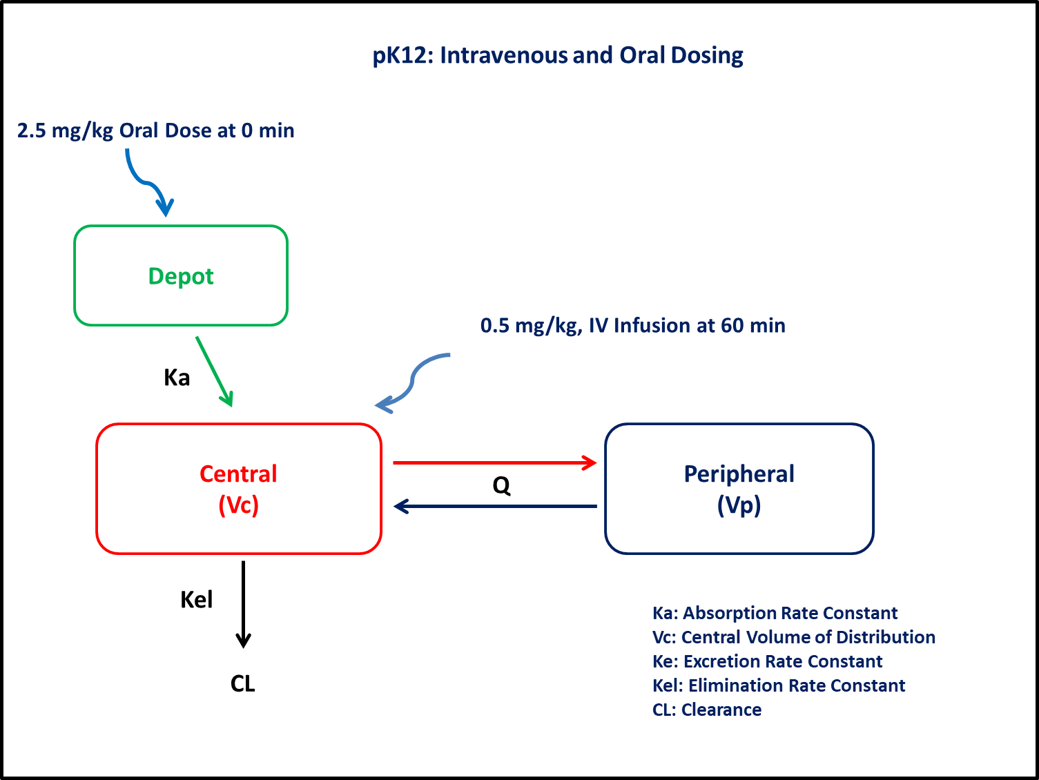
PK12 - Intravenous and oral dosing
1 Background
To determine (oral) bioavailability, the drug is administered by both oral and intravenous routes. The administration is generally done in a crossover manner at different times, separated by a washout period. But if the drug follows a time-dependent clearance (and if the washout period is long), then it may affect the results. To avoid this situation, the doses can be administered semi-simultaneously, separated by a small time up to 1 hour.
In the current study, the test drug was administered orally, followed by a constant rate infusion (reference) for 15 minutes at 60 minutes.
- Structural model - Two compartment model with first order absorption and elimination
- Route of administration - Oral and IV given simultaneously
- Dosage Regimen - 2.5 mg Oral and 0.5 mg IV infusion for 15 minutes
- Number of Subjects - 1
2 Learning Outcomes
This exercise demonstrates the bioavailability of a compound administered semi-simultaneously by oral and intravenous routes.
3 Objectives
- To build a two-compartment model for semi-simultaneous oral and intravenous administration
- To design a semi-simultaneous dosage regimen
- To simulate and plot a single subject with predefined time points.
4 Libraries
Load the necessary libraries.
5 Model definition
Note the expression of the model parameters with helpful comments. The model is expressed with differential equations. Residual variability is a proportional error model.
A two compartment model with oral absorption is built for a semi-simultaneous administration of an oral dose followed by intravenous infusion.
pk_12 = @model begin
    @metadata begin
        desc = "Two Compartment Model"
        timeu = u"minute"
    end

    @param begin
        """
        Absorption Rate Constant (min⁻¹)
        """
        tvka ∈ RealDomain(lower = 0)
        """
        Clearance (L/min/kg)
        """
        tvcl ∈ RealDomain(lower = 0)
        """
        Inter-compartmental distribution (L/kg)
        """
        tvq ∈ RealDomain(lower = 0)
        """
        Volume of Central Compartment (L/kg)
        """
        tvvc ∈ RealDomain(lower = 0)
        """
        Volume of Peripheral Compartment (L/kg)
        """
        tvvp ∈ RealDomain(lower = 0)
        """
        Lag time (min)
        """
        tvlag ∈ RealDomain(lower = 0)
        """
        Bioavailability
        """
        tvF ∈ RealDomain(lower = 0)
        Ω_ka ∈ RealDomain(lower = 0.0001)
        Ω_cl ∈ RealDomain(lower = 0.0001)
        Ω_q ∈ RealDomain(lower = 0.0001)
        Ω_vc ∈ RealDomain(lower = 0.0001)
        Ω_vp ∈ RealDomain(lower = 0.0001)
        Ω_lag ∈ RealDomain(lower = 0.0001)
        Ω_F ∈ RealDomain(lower = 0.0001)
        """
        Proportional RUV
        """
        σ²_prop ∈ RealDomain(lower = 0)
    end

    @random begin
        η_ka ~ Normal(0, sqrt(Ω_ka))
        η_cl ~ Normal(0, sqrt(Ω_cl))
        η_q ~ Normal(0, sqrt(Ω_q))
        η_vc ~ Normal(0, sqrt(Ω_vc))
        η_vp ~ Normal(0, sqrt(Ω_vp))
        η_lag ~ Normal(0, sqrt(Ω_lag))
        η_F ~ Normal(0, sqrt(Ω_F))
    end

    @pre begin
        CL = tvcl * exp(η_cl)
        Q = tvq * exp(η_q)
        Vc = tvvc * exp(η_vc)
        Vp = tvvp * exp(η_vp)
        Ka = tvka * exp(η_ka)
    end

    @dosecontrol begin
        lags = (Depot = tvlag * exp(η_lag),)
        bioav = (Depot = tvF * exp(η_F),)
    end

    @dynamics Depots1Central1Periph1

    @derived begin
        cp = @. 1000 * (Central / Vc)
        """
        Observed Concentrations (μg/L)
        """
        dv ~ ProportionalNormal.(cp, sqrt(σ²_prop))
    end
end
┌ Warning: Variable `cp` is defined in the `@derived` block using `=` and hence `cp` is not used for model fitting but only returned when simulating: │ If `cp` is a random variable, it must be defined in the `@derived` block using `~`; │ if `cp` should be returned when simulating, it should be defined in the `@observed` block using `=`; │ if `cp` is an intermediate quantity that should not be returned when simulating, it should be defined using `:=`. └ @ Pumas ~/run/_work/PumasTutorials.jl/PumasTutorials.jl/custom_julia_depot/packages/Pumas/GZeMg/src/dsl/model_macro.jl:2351
PumasModel
  Parameters: tvka, tvcl, tvq, tvvc, tvvp, tvlag, tvF, Ω_ka, Ω_cl, Ω_q, Ω_vc, Ω_vp, Ω_lag, Ω_F, σ²_prop
  Random effects: η_ka, η_cl, η_q, η_vc, η_vp, η_lag, η_F
  Covariates:
  Dynamical system variables: Depot, Central, Peripheral
  Dynamical system type: Closed form
  Derived: cp, dv
  Observed: cp, dv
6 Initial Estimates of Model Parameters
The model parameters for simulation are the following. Note that tv represents the typical value for parameters.
Ka- Absorption Rate Constant (min⁻¹)Cl- Clearance (L/min/kg)Q- Inter-compartmental distribution (L/kg)Vc- Volume of Central Compartment (L/kg)Vp- Volume of Peripheral Compartment (L/kg)lag- Lag time (min)F- Bioavailabilityσ- Residual Error
param = (
    tvka = 0.103,
    tvcl = 0.015,
    tvq = 0.021,
    tvvc = 0.121,
    tvvp = 0.276,
    tvlag = 4.68,
    tvF = 0.046,
    Ω_ka = 0.01,
    Ω_cl = 0.01,
    Ω_q = 0.01,
    Ω_vc = 0.01,
    Ω_vp = 0.01,
    Ω_lag = 0.01,
    Ω_F = 0.01,
    σ²_prop = 0.04,
)
7 Dosage Regimen
Dosage Regimen - 2.5 mg/kg orally followed by a 15 minute intravenous infusion of 0.5 mg/kg starting 60 minutes after oral dosing, administered to a single subject (sub1).
ev_oral = DosageRegimen(2.5, time = 0, cmt = 1)1×10 DataFrame
| Row | time | cmt | amt | evid | ii | addl | rate | duration | ss | route |
|---|---|---|---|---|---|---|---|---|---|---|
| Float64 | Int64 | Float64 | Int8 | Float64 | Int64 | Float64 | Float64 | Int8 | NCA.Route | |
| 1 | 0.0 | 1 | 2.5 | 1 | 0.0 | 0 | 0.0 | 0.0 | 0 | NullRoute |
ev_inf = DosageRegimen(0.5, time = 60, cmt = 2, duration = 15)1×10 DataFrame
| Row | time | cmt | amt | evid | ii | addl | rate | duration | ss | route |
|---|---|---|---|---|---|---|---|---|---|---|
| Float64 | Int64 | Float64 | Int8 | Float64 | Int64 | Float64 | Float64 | Int8 | NCA.Route | |
| 1 | 60.0 | 2 | 0.5 | 1 | 0.0 | 0 | 0.0333333 | 15.0 | 0 | NullRoute |
ev1 = DosageRegimen(ev_oral, ev_inf)2×10 DataFrame
| Row | time | cmt | amt | evid | ii | addl | rate | duration | ss | route |
|---|---|---|---|---|---|---|---|---|---|---|
| Float64 | Int64 | Float64 | Int8 | Float64 | Int64 | Float64 | Float64 | Int8 | NCA.Route | |
| 1 | 0.0 | 1 | 2.5 | 1 | 0.0 | 0 | 0.0 | 0.0 | 0 | NullRoute |
| 2 | 60.0 | 2 | 0.5 | 1 | 0.0 | 0 | 0.0333333 | 15.0 | 0 | NullRoute |
8 Single-individual that receives the defined dose
sub1 = Subject(id = 1, events = ev1)Subject
ID: 1
Events: 29 Single-Subject Simulation
Simulate plasma concentrations with specific observation time points
Initialize the random number generator with a seed for reproducibility of the simulation.
Random.seed!(123)Define the timepoints at which concentration values will be simulated.
sim_s1 = simobs(
    pk_12,
    sub1,
    param,
    obstimes = [6, 10, 15, 20, 30, 45, 60, 63, 66, 75, 80, 90, 107, 119, 134, 150],
)
SimulatedObservations
Simulated variables: cp, dv
Time: [6, 10, 15, 20, 30, 45, 60, 63, 66, 75, 80, 90, 107, 119, 134, 150]10 Visualize Results
@chain DataFrame(sim_s1) begin
    dropmissing(:cp)
    data(_) *
    mapping(:time => "Time (minutes)", :cp => "Concentration (μg/L)") *
    visual(Lines; linewidth = 4)
    draw(;
        figure = (; fontsize = 22),
        axis = (;
            yscale = Makie.pseudolog10,
            yticks = map(i -> 10^i, 1:0.5:3),
            ytickformat = x -> string.(round.(x; digits = 1)),
            xticks = 0:20:160,
        ),
    )
end
11 Perform a Population Simulation
We perform a population simulation with 40 participants.
This code demonstrates how to write the simulated concentrations to a comma separated file (.csv).
par = (
    tvka = 0.103,
    tvcl = 0.015,
    tvq = 0.021,
    tvvc = 0.121,
    tvvp = 0.276,
    tvlag = 4.68,
    tvF = 0.046,
    Ω_ka = 0.0625,
    Ω_cl = 0.0016,
    Ω_q = 0.0169,
    Ω_vc = 0.0064,
    Ω_vp = 0.0121,
    Ω_lag = 0.0144,
    Ω_F = 0.0144,
    σ²_prop = 0.04,
)

ev1 = DosageRegimen([2.5, 0.5], time = [0, 60], cmt = [1, 2], duration = [0, 15])
pop = map(i -> Subject(id = i, events = ev1), 1:40)

Random.seed!(1234)
pop_sim = simobs(pk_12, pop, par, obstimes = 0:1:150)
pkdata_12_sim = DataFrame(pop_sim)
#CSV.write("pk_12_sim.csv", pkdata_12_sim)
12 Conclusion
This tutorial showed how to build a two-compartment model for semi-simultaneous oral and intravenous administration and perform a single subject and population simulation.