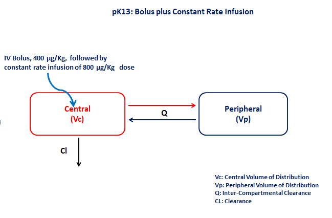
PK13 - Bolus plus constant rate infusion

1 Background

Structural model - Two compartment model with first order elimination
Route of administration - IV-Bolus and IV-Infusion given simultaneously
Dosage Regimen - 400 μg/kg IV-Bolus and 800 μg/kg IV-Infusion for 26 minutes
Number of Subjects - 1

2 Learning Outcome

Write the differential equation for a two-compartment model in terms of Clearance and Volume
Simulate data for a bolus dose followed by a constant rate infusion regimen
Observe how the administration of a loading dose helps to achieve therapeutic concentrations faster

3 Objective

The objective of this exercise is to simulate data from a bolus followed by a constant rate infusion using a differential equation model.

4 Libraries

Call the necessary libraries to get started

using Random
using Pumas
using PumasUtilities
using AlgebraOfGraphics
using CairoMakie
using CSV
using DataFramesMeta
using Dates

5 Model

The given data follows a two compartment model in which the IV Bolus and IV-Infusion are administered at time=0

pk_13 = @model begin
    @metadata begin
        desc = "Two Compartment Model"
        timeu = u"minute"
    end

    @param begin
        """
        Clearance (L/min/kg)
        """
        tvcl ∈ RealDomain(lower = 0)
        """
        Volume of Central Compartment (L/kg)
        """
        tvvc ∈ RealDomain(lower = 0)
        """
        Inter-compartmental Clearance (L/min/kg)
        """
        tvq ∈ RealDomain(lower = 0)
        """
        Volume of Peripheral Compartment (L/kg)
        """
        tvvp ∈ RealDomain(lower = 0)
        Ω ∈ PDiagDomain(4)
        """
        Proportional RUV
        """
        σ²_prop ∈ RealDomain(lower = 0)
        """
        Additive RUV
        """
        σ²_add ∈ RealDomain(lower = 0)
    end

    @random begin
        η ~ MvNormal(Ω)
    end

    @pre begin
        Cl = tvcl * exp(η[1])
        Vc = tvvc * exp(η[2])
        Q = tvq * exp(η[3])
        Vp = tvvp * exp(η[4])
    end

    @dynamics begin
        Central' = -(Cl / Vc) * Central - (Q / Vc) * Central + (Q / Vp) * Peripheral
        Peripheral' = (Q / Vc) * Central - (Q / Vp) * Peripheral
    end

    @derived begin
        cp = @. Central / Vc
        """
        Observed Concentrations (μg/L)
        """
        dv ~ @. Normal(cp, sqrt((cp * σ²_prop)^2 + σ²_add^2))
    end
end

PumasModel
  Parameters: tvcl, tvvc, tvq, tvvp, Ω, σ²_prop, σ²_add
  Random effects: η
  Covariates:
  Dynamical system variables: Central, Peripheral
  Dynamical system type: Nonlinear ODE
  Derived: cp, dv
  Observed: cp, dv

6 Parameters

Cl - Clearance of central compartment (L/min/kg)
Vc - Volume of central compartment (L/kg)
Q - Inter-compartmental clearance (L/min/kg)
Vp - Volume of peripheral compartment (L/kg)
Ω - Between Subject Variability
σ - Residual Unexplained Variability

param = (
    tvcl = 0.344708,
    tvvc = 2.8946,
    tvq = 0.178392,
    tvvp = 2.18368,
    Ω = Diagonal([0.04, 0.04, 0.04, 0.04]),
    σ²_prop = 0.0571079,
    σ²_add = 0.1,
)

7 Dosage Regimen

Single dose of 400 μg/kg given as an IV-Bolus at time=0
Single dose of 800 μg/kg given as an IV-Infusion for 26 minutes at time=0

ev1 = DosageRegimen(400, time = 0, cmt = 1)

1×10 DataFrame

Row	time	cmt	amt	evid	ii	addl	rate	duration	ss	route
	Float64	Int64	Float64	Int8	Float64	Int64	Float64	Float64	Int8	NCA.Route
1	0.0	1	400.0	1	0.0	0	0.0	0.0	0	NullRoute

ev2 = DosageRegimen(800, time = 0, cmt = 1, rate = 30.769)

1×10 DataFrame

Row	time	cmt	amt	evid	ii	addl	rate	duration	ss	route
	Float64	Int64	Float64	Int8	Float64	Int64	Float64	Float64	Int8	NCA.Route
1	0.0	1	800.0	1	0.0	0	30.769	26.0002	0	NullRoute

ev3 = DosageRegimen(ev1, ev2)

2×10 DataFrame

Row	time	cmt	amt	evid	ii	addl	rate	duration	ss	route
	Float64	Int64	Float64	Int8	Float64	Int64	Float64	Float64	Int8	NCA.Route
1	0.0	1	400.0	1	0.0	0	0.0	0.0	0	NullRoute
2	0.0	1	800.0	1	0.0	0	30.769	26.0002	0	NullRoute

sub1 = Subject(id = 1, events = ev3)

Subject
  ID: 1
  Events: 2

8 Simulation

We will simulate the plasma concentration at the pre-specified time points.

Random.seed!(123)

The random effects are zero’ed out since we are simulating means

zfx = zero_randeffs(pk_13, sub1, param)

(η = [0.0, 0.0, 0.0, 0.0],)

sim_sub1 = simobs(
    pk_13,
    sub1,
    param,
    zfx,
    obstimes = [
        2,
        5,
        10,
        15,
        20,
        25,
        30,
        33,
        35,
        37,
        40,
        45,
        50,
        60,
        70,
        90,
        110,
        120,
        150,
    ],
)

SimulatedObservations
  Simulated variables: cp, dv
  Time: [2, 5, 10, 15, 20, 25, 30, 33, 35, 37, 40, 45, 50, 60, 70, 90, 110, 120, 150]

9 Visualization

@chain DataFrame(sim_sub1) begin
    dropmissing(:cp)
    data(_) *
    mapping(:time => "Time (min)", :cp => "PK13 Concentration (μg/L)") *
    visual(Lines, linewidth = 4)
    draw(;
        axis = (;
            yscale = log10,
            xticks = 0:20:160,
            ytickformat = x -> string.(round.(x; digits = 1)),
            ygridwidth = 3,
            yminorticksvisible = true,
            yminorgridvisible = true,
            yminorticks = IntervalsBetween(10),
        ),
        figure = (; fontsize = 22),
    )
end

par = (
    tvcl = 0.344708,
    tvvc = 2.8946,
    tvq = 0.178392,
    tvvp = 2.18368,
    Ω = Diagonal([0.09, 0.04, 0.0225, 0.0125]),
    # tvCMixRatio = 1.00693,
    σ²_prop = 0.0571079,
    σ²_add = 0.2,
)

ev = DosageRegimen([400, 800], time = 0, cmt = 1, duration = [0, 26])
pop = map(i -> Subject(id = i, events = ev), 1:48)

Random.seed!(1234)
pop_sim = simobs(
    pk_13,
    pop,
    par,
    obstimes = [
        2,
        5,
        10,
        15,
        20,
        25,
        30,
        33,
        35,
        37,
        40,
        45,
        50,
        60,
        70,
        90,
        110,
        120,
        150,
    ],
)

sim_plot(pop_sim)
df_sim = DataFrame(pop_sim)
#CSV.write("pk_13.csv", df_sim)