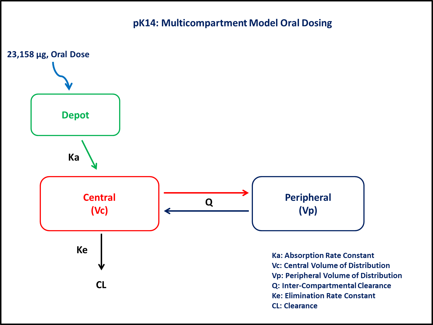
PK14 - Multi-compartment model oral dosing

1 Background

• Structural model - Two compartment linear elimination and first order absorption with lagtime
• Route of administration - Oral
• Dosage regimens - 23,158 μg single dose
• Subject - 1

PK14 Model Graph

2 Learning Outcome

In this model, we will simulate an oral dose to understand the disposition of a drug following lag time in absorption

3 Objectives

In this tutorial, you will learn how to build a two compartment model with lag time in oral absorption and to simulate the model for a single subject.

4 Libraries

Call the necessary libraries to get started

using Random
using Pumas
using PumasUtilities
using AlgebraOfGraphics
using CairoMakie
using CSV
using DataFramesMeta
using Dates

5 Model

In this two compartment model, we administer doses to the Depot and Central compartments.

pk_14 = @model begin
    @metadata begin
        desc = "Two Compartment Model"
        timeu = u"hr"
    end

    @param begin
        """
        Absorption Rate Constant (hr⁻¹)
        """
        tvka ∈ RealDomain(lower = 0)
        """
        Volume of Central Compartment (L)
        """
        tvvc ∈ RealDomain(lower = 0)
        """
        Volume of Peripheral Compartment (L)
        """
        tvvp ∈ RealDomain(lower = 0)
        """
        Clearance (L/hr)
        """
        tvcl ∈ RealDomain(lower = 0)
        """
        Intercompartmental Clearance (L/hr)
        """
        tvq ∈ RealDomain(lower = 0)
        """
        Lagtime (hr)
        """
        tvlag ∈ RealDomain(lower = 0)
        Ω ∈ PDiagDomain(4)
        """
        Proportional RUV
        """
        σ²_prop ∈ RealDomain(lower = 0)
    end

    @random begin
        η ~ MvNormal(Ω)
    end

    @pre begin
        Ka = tvka * exp(η[1])
        Vc = tvvc * exp(η[2])
        Vp = tvvp * exp(η[3])
        CL = tvcl * exp(η[4])
        Q = tvq
    end

    @dosecontrol begin
        lags = (Depot = tvlag,)
    end

    @dynamics Depots1Central1Periph1

    @derived begin
        cp = @. Central / Vc
        """
        Observed Concentrations (μg/L)
        """
        dv ~ @. Normal(cp, sqrt(cp^2 * σ²_prop))
    end
end

PumasModel
  Parameters: tvka, tvvc, tvvp, tvcl, tvq, tvlag, Ω, σ²_prop
  Random effects: η
  Covariates: 
  Dynamical system variables: Depot, Central, Peripheral
  Dynamical system type: Closed form
  Derived: cp, dv
  Observed: cp, dv

6 Parameters

Parameters provided for simulation. Note that tv represents the typical value for parameters.

• Ka - Absorption rate constant (hr⁻¹)
• Vc - Volume of central compartment (L)
• Vp - Volume of peripheral Compartmental (L)
• CL - Clearance (L/hr)
• Q - Intercompartmental clearance (L/hr)
• lag - Absorption lag time (hr)

param = (
    tvka = 10,
    tvvc = 82.95,
    tvcl = 54.87,
    tvq = 10.55,
    tvlag = 0.078,
    tvvp = 107.9,
    Ω = Diagonal([0.04, 0.04, 0.04, 0.04]),
    σ²_prop = 0.0125,
)

7 Dosage Regimen

A single subject receives an oral dose of 23158 μg at time=0

ev1 = DosageRegimen(23158, time = 0, cmt = 1)

1×10 DataFrame

Row	time	cmt	amt	evid	ii	addl	rate	duration	ss	route
	Float64	Int64	Float64	Int8	Float64	Int64	Float64	Float64	Int8	NCA.Route
1	0.0	1	23158.0	1	0.0	0	0.0	0.0	0	NullRoute

sub1 = Subject(id = 1, events = ev1)

Subject
  ID: 1
  Events: 1

8 Simulation

Let’s simulate plasma concentration after oral dosing

Random.seed!(123)

The random effects are zero’ed out since we are simulating means

zfx = zero_randeffs(pk_14, sub1, param)

(η = [0.0, 0.0, 0.0, 0.0],)

sim_sub1 = simobs(pk_14, sub1, param, zfx, obstimes = 0.08:0.01:25)

SimulatedObservations
  Simulated variables: cp, dv
  Time: 0.08:0.01:25.0

9 Visualization

@chain DataFrame(sim_sub1) begin
    dropmissing(:cp)
    data(_) *
    mapping(:time => "Time (hours)", :cp => "Concentration (μg/L)") *
    visual(Lines, linewidth = 4)
    draw(;
        axis = (;
            yscale = log10,
            yticks = map(i -> 10^i, 0:0.5:2),
            ytickformat = i -> (@. string(round(i; digits = 1))),
            xticks = 0:5:25,
        ),
        figure = (; fontsize = 22),
    )
end

10 Population simulation

par = (
    tvka = 10,
    tvvc = 82.95,
    tvcl = 54.87,
    tvq = 10.55,
    tvlag = 0.078,
    tvvp = 107.9,
    Ω = Diagonal([0.0152, 0.0426, 0.092, 0.0158]),
    σ²_prop = 0.03,
)

ev1 = DosageRegimen(23158, time = 0, cmt = 1)
pop = map(i -> Subject(id = i, events = ev1), 1:68)

Random.seed!(1234)
sim_pop = simobs(
    pk_14,
    pop,
    par,
    obstimes = [0.08, 0.16, 0.25, 0.5, 1, 1.5, 2, 3, 4, 6, 8, 12, 24, 25],
)
sim_plot(sim_pop, yaxis = :log)

df_sim = DataFrame(sim_pop);

#CSV.write("pk_14.csv", df_sim)