using PumasUtilities
using Random
using Pumas
using CairoMakie
using AlgebraOfGraphics
using CSV
using DataFramesMeta
using Dates
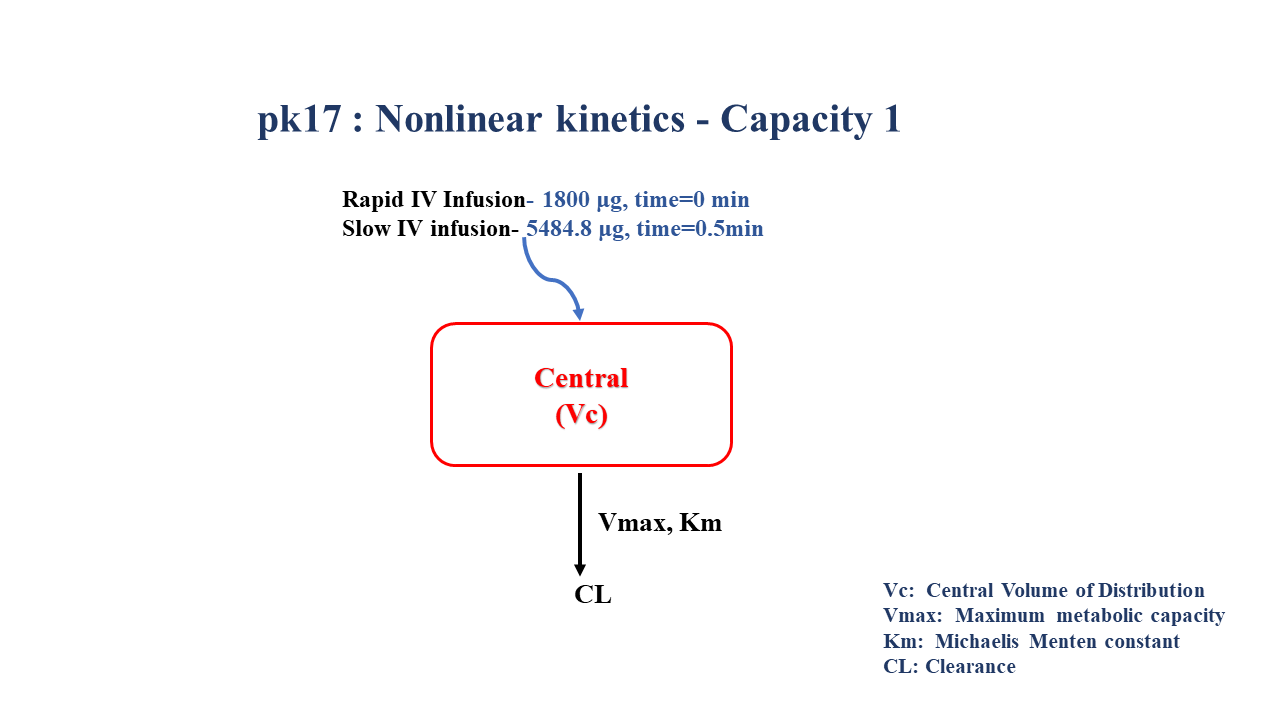
PK17 - Nonlinear Kinetics (Capacity I-IV, Flow, Hetero/Autoinduction)
1 Background
- Structural model - One compartment non-linear elimination
- Route of administration - IV infusion
- Dosage Regimen - 1800 μg rapid IV, 5484.8 μg slow IV
- Number of Subjects - 1
2 Learning Outcomes
This tutorial demonstrates simulating plasma concentration data following multiple intravenous infusions from a one compartment model taking into consideration non-linear elimination parameters.
3 Objectives
To build a one-compartment model for capacity limited kinetics, simulate the model for a single subject given multiple IV infusions, and subsequently perform a simulation for a population.
4 Libraries
Load the necessary libraries.
5 Model definition
Note the expression of the model parameters with helpful comments. The model is expressed with differential equations. Residual variability is a proportional error model.
In this one compartment model following linear elimination, multiple IV infusions are administered into the central compartment.
5.1 Linear Model
pk_17_ln = @model begin
    @metadata begin
        desc = "Linear One Compartment Model"
        timeu = u"minute"
    end

    @param begin
        """
        Clearance (mL/min)
        """
        tvcl ∈ RealDomain(lower = 0)
        """
        Volume of Distribution (mL)
        """
        tvvc ∈ RealDomain(lower = 0)
        Ω ∈ PDiagDomain(2)
        """
        Additive RUV
        """
        σ ∈ RealDomain(lower = 0)
    end

    @random begin
        η ~ MvNormal(Ω)
    end

    @pre begin
        Cl = tvcl * exp(η[1])
        Vc = tvvc * exp(η[2])
    end

    @dynamics begin
        Central' = -(Cl / Vc) * Central
    end

    @derived begin
        cp = @. Central / Vc
        """
        Observed Concentration (μg/ml)
        """
        dv ~ @. Normal(cp, σ)
    end
end
┌ Warning: Variable `cp` is defined in the `@derived` block using `=` and hence `cp` is not used for model fitting but only returned when simulating: │ If `cp` is a random variable, it must be defined in the `@derived` block using `~`; │ if `cp` should be returned when simulating, it should be defined in the `@observed` block using `=`; │ if `cp` is an intermediate quantity that should not be returned when simulating, it should be defined using `:=`. └ @ Pumas ~/run/_work/PumasTutorials.jl/PumasTutorials.jl/custom_julia_depot/packages/Pumas/GZeMg/src/dsl/model_macro.jl:2351
PumasModel
  Parameters: tvcl, tvvc, Ω, σ
  Random effects: η
  Covariates:
  Dynamical system variables: Central
  Dynamical system type: Matrix exponential
  Derived: cp, dv
  Observed: cp, dv
5.2 Define Initial Estimates of Model Parameters - Linear Model
The Parameters are as given below. Note that tv represents the typical value for parameters.
Cl- Clearance (mL/min)Vc- Volume of Distribution of Central Compartment (mL)Ω- Between Subject Variabilityσ- Residual Error
param_ln = (tvcl = 43.3, tvvc = 1380, Ω = Diagonal([0.01, 0.01]), σ = 0.00)5.3 Michaelis Menten Model
In this one compartment model following non-linear elimination, multiple IV infusions are administered into the central compartment.
pk_17_mm = @model begin
    @metadata begin
        desc = "Michaelis Menten - One Compartment Model"
        timeu = u"hr"
    end

    @param begin
        """
        Maximum Metabolic Capacity (μg/min)
        """
        tvvmax ∈ RealDomain(lower = 0)
        """
        Michaelis-Menten Constant (μg/mL)
        """
        tvkm ∈ RealDomain(lower = 0)
        """
        Volume of Distribution (mL)
        """
        tvvc ∈ RealDomain(lower = 0)
        Ω ∈ PDiagDomain(3)
        """
        Additive RUV
        """
        σ ∈ RealDomain(lower = 0)
    end

    @random begin
        η ~ MvNormal(Ω)
    end

    @pre begin
        Vmax = tvvmax * exp(η[1])
        Km = tvkm * exp(η[2])
        Vc = tvvc * exp(η[3])
    end

    @dynamics begin
        Central' = -(Vmax / (Km + (Central / Vc))) * (Central / Vc)
    end

    @derived begin
        cp = @. Central / Vc
        """
        Observed Concentration (μg/ml)"
        """
        dv ~ @. ProportionalNormal(cp, σ)
    end
end
┌ Warning: Variable `cp` is defined in the `@derived` block using `=` and hence `cp` is not used for model fitting but only returned when simulating: │ If `cp` is a random variable, it must be defined in the `@derived` block using `~`; │ if `cp` should be returned when simulating, it should be defined in the `@observed` block using `=`; │ if `cp` is an intermediate quantity that should not be returned when simulating, it should be defined using `:=`. └ @ Pumas ~/run/_work/PumasTutorials.jl/PumasTutorials.jl/custom_julia_depot/packages/Pumas/GZeMg/src/dsl/model_macro.jl:2351
PumasModel
  Parameters: tvvmax, tvkm, tvvc, Ω, σ
  Random effects: η
  Covariates:
  Dynamical system variables: Central
  Dynamical system type: Nonlinear ODE
  Derived: cp, dv
  Observed: cp, dv
5.4 Define Initial Estimates of Model Parameters- Michaelis Menten Model
The Parameters are as given below. Note that tv represents the typical value for parameters.
Vmax- Maximum Metabolic Capacity (μg/min)Km- Michaelis-Menten Constant (μg/mL)Vc- Volume of Distribution of Central Compartment (mL)Ω- Between Subject Variabilityσ- Residual Error
param_mm = (
    tvvmax = 124.451,
    tvkm = 0.981806,
    tvvc = 1350.61,
    Ω = Diagonal([0.01, 0.01, 0.01]),
    σ = 0.007,
)
6 Dosage Regimen
A single subject received a rapid infusion of 1800 μg over 0.5 minutes, followed by 5484.8 μg over 39.63 minutes.
DR = DosageRegimen([1800, 5484.8], time = [0, 0.5], cmt = [1, 1], duration = [0.5, 39.63])2×10 DataFrame
| Row | time | cmt | amt | evid | ii | addl | rate | duration | ss | route |
|---|---|---|---|---|---|---|---|---|---|---|
| Float64 | Int64 | Float64 | Int8 | Float64 | Int64 | Float64 | Float64 | Int8 | NCA.Route | |
| 1 | 0.0 | 1 | 1800.0 | 1 | 0.0 | 0 | 3600.0 | 0.5 | 0 | NullRoute |
| 2 | 0.5 | 1 | 5484.8 | 1 | 0.0 | 0 | 138.4 | 39.63 | 0 | NullRoute |
7 Single-individual that receives the defined dose
s1 = Subject(id = "ID:1 Linear Kinetics", events = DR)Subject
ID: ID:1 Linear Kinetics
Events: 2s2 = Subject(id = "ID:2 Michaelis-Menten Kinetics", events = DR)Subject
ID: ID:2 Michaelis-Menten Kinetics
Events: 28 Single-Subject Simulation
Simulate for plasma concentration for a single subject for specific observation time points after multiple IV infusion doses.
Initialize the random number generator with a seed for reproducibility of the simulation.
8.1 Linear model
Random.seed!(1234)Define the timepoints at which concentration values will be simulated.
sim_ln = simobs(pk_17_ln, s1, param_ln, obstimes = 0.0:0.01:80.35)SimulatedObservations
Simulated variables: cp, dv
Time: 0.0:0.01:80.358.2 Michaelis Menten Model
Define the timepoints at which concentration values will be simulated.
sim_mm = simobs(pk_17_mm, s2, param_mm, obstimes = 0.0:0.01:80.35)SimulatedObservations
Simulated variables: cp, dv
Time: 0.0:0.01:80.359 Visualize Results
plt_ln = @chain DataFrame(sim_ln) begin
    dropmissing(:cp)
    data(_) *
    mapping(:time => "Time (minutes)", :cp => "Concentration (μg/mL)", color = :id => "") *
    visual(Lines; linewidth = 4)
end

plt_mm = @chain DataFrame(sim_mm) begin
    dropmissing(:cp)
    data(_) *
    mapping(:time => "Time (minutes)", :cp => "Concentration (μg/mL)", color = :id => "") *
    visual(Lines; linewidth = 4)
end

draw(
    plt_ln + plt_mm;
    axis = (; xticks = 0:10:90),
    figure = (; fontsize = 22),
    legend = (; position = :bottom),
)
10 Perform a Population Simulation
We perform a population simulation with 45 participants.
This code demonstrates how to write the simulated concentrations to a comma separated file (.csv).
param = (
    tvvmax = 124.451,
    tvkm = 0.981806,
    tvvc = 1350.61,
    Ω = Diagonal([0.04, 0.025, 0.0025]),
    σ = 0.0573191,
)

DR = DosageRegimen([1800, 5484.8], time = [0, 0.5], cmt = [1, 1], duration = [0.5, 39.63])
pop = map(i -> Subject(id = i, events = DR), 1:45)

Random.seed!(123)
pop_sim = simobs(
    pk_17_mm,
    pop,
    param,
    obstimes = [
        0.1,
        5.38,
        10.33,
        15.3,
        20.35,
        23.13,
        28.15,
        33.18,
        38.23,
        40.62,
        45.25,
        50.08,
        60.42,
        80.35,
    ],
)

pkdata_17_sim = DataFrame(pop_sim)
#CSV.write("pk_17_sim.csv", pkdata_17_sim);
11 Conclusion
This tutorial showed how to build a one-compartment model for IV infusion, taking into consideration non-linear elimination parameters, and perform a single subject and population simulation.