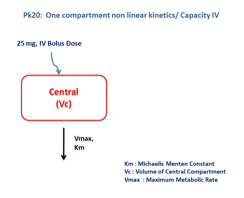
PK20 - One-compartment model with capacity limited elimination for IV bolus

1 Background

Structural Model - One Compartment Model with nonlinear elimination.
Route of administration - IV bolus
Dosage Regimen - 25 mg and 100 mg
Number of Subjects - 2

2 Learning Outcome

This exercise demonstrates simulating IV bolus with different dosage regimens and different Vmax and Km values with capacity limited elimination from a one compartment model.

3 Objectives

To build a one-compartment model for an IV bolus dose with capacity limited elimination, simulate the model for each subject, and subsequently perform a simulation for a population.

4 Libraries

Load the necessary libraries.

using PumasUtilities
using Random
using Pumas
using CairoMakie
using AlgebraOfGraphics
using CSV
using DataFramesMeta
using Dates

5 Model definition

Note the expression of the model parameters with helpful comments. The model is expressed with differential equations. Residual variability is a proportional error model.

pk_20 = @model begin
    @metadata begin
        desc = "One Compartment Model - Nonlinear Elimination"
        timeu = u"hr"
    end

    @param begin
        """
        Volume of Central Compartment (L)
        """
        tvvc ∈ RealDomain(lower = 0)
        """
        Michaelis menten Constant (μg/L)
        """
        tvkm ∈ RealDomain(lower = 0)
        """
        Maximum Rate of Metabolism (μg/hr)
        """
        tvvmax ∈ RealDomain(lower = 0)
        Ω ∈ PDiagDomain(3)
        """
        Proportional RUV
        """
        σ_prop ∈ RealDomain(lower = 0)
    end

    @random begin
        η ~ MvNormal(Ω)
    end

    @pre begin
        Vc = tvvc * exp(η[1])
        Km = tvkm * exp(η[2])
        Vmax = tvvmax * exp(η[3])
    end

    @dynamics begin
        Central' = -(Vmax * (Central / Vc) / (Km + (Central / Vc)))
    end

    @derived begin
        cp = @. Central / Vc
        """
        Observed Concentration (μg/L)
        """
        dv ~ @. Normal(cp, cp * σ_prop)
    end
end

PumasModel
  Parameters: tvvc, tvkm, tvvmax, Ω, σ_prop
  Random effects: η
  Covariates: 
  Dynamical system variables: Central
  Dynamical system type: Nonlinear ODE
  Derived: cp, dv
  Observed: cp, dv

6 Initial Estimates of Model Parameters

The model parameters for simulation are the following. Note that tv represents the typical value for parameters.

Km - Michaelis menten Constant (μg/L)
Vc - Volume of Central Compartment (L),
Vmax - Maximum rate of metabolism (μg/hr),
Ω - Between Subject Variability,
σ - Residual error

Note

A vector of model parameter values is defined.

param1 are the parameter values for Subject 1
param2 are the parameter values for Subject 2

param1 = (
    tvkm = 261.736,
    tvvmax = 36175.1,
    tvvc = 48.9892,
    Ω = Diagonal([0.01, 0.01, 0.01]),
    σ_prop = 0.01,
)

param2 = (param1..., tvkm = 751.33)

Merge both parameters

param = vcat(param1, param2)

7 Define the Dosage Regimen and Subjects

Subject 1 - receives an IV dose of 25 mg or 25000 μg
Subject 2 - receives an IV dose of 100 mg or 100000 μg

ev1 = DosageRegimen(25000, time = 0, cmt = 1)

1×10 DataFrame

Row	time	cmt	amt	evid	ii	addl	rate	duration	ss	route
	Float64	Int64	Float64	Int8	Float64	Int64	Float64	Float64	Int8	NCA.Route
1	0.0	1	25000.0	1	0.0	0	0.0	0.0	0	NullRoute

sub1 = Subject(id = 1, events = ev1, time = 0.01:0.01:2, observations = (; dv = nothing,))

Subject
  ID: 1
  Events: 1
  Observations: dv: (n=200)

ev2 = DosageRegimen(100000, time = 0, cmt = 1)

1×10 DataFrame

Row	time	cmt	amt	evid	ii	addl	rate	duration	ss	route
	Float64	Int64	Float64	Int8	Float64	Int64	Float64	Float64	Int8	NCA.Route
1	0.0	1	100000.0	1	0.0	0	0.0	0.0	0	NullRoute

sub2 = Subject(id = 2, events = ev2, time = 0.01:0.01:8, observations = (; dv = nothing,))

Subject
  ID: 2
  Events: 1
  Observations: dv: (n=800)

pop = [sub1, sub2]

Population
  Subjects: 2
  Observations: dv

8 Single-Subject Simulation

Simulate the plasma drug concentration for the two subjects

Initialize the random number generator with a seed for reproducibility of the simulation.

Random.seed!(123)

sim = map(((subject, paramᵢ),) -> simobs(pk_20, subject, paramᵢ), zip(pop, param))

Simulated population (Vector{<:Subject})
  Simulated subjects: 2
  Simulated variables: cp, dv

9 Visualize Results

@chain DataFrame(sim) begin
    dropmissing(:cp)
    data(_) *
    mapping(
        :time => "Time (hours)",
        :cp => "Concentration (μg/L)";
        color = :id => "Subject",
    ) *
    visual(Lines; linewidth = 4)
    draw(;
        figure = (; fontsize = 22),
        axis = (; xticks = 0:1:8),
        legend = (; position = :bottom),
    )
end

10 Population Simulation

We perform a population simulation with 45 participants.

This code demonstrates how to write the simulated concentrations to a comma separated file (.csv).

par1 = (
    tvkm = 261.736,
    tvvmax = 36175.1,
    tvvc = 48.9892,
    Ω = Diagonal([0.09, 0.04, 0.0225]),
    σ_prop = 0.0927233,
)

par2 = (
    tvkm = 751.33,
    tvvmax = 36175.1,
    tvvc = 48.9892,
    Ω = Diagonal([0.04, 0.09, 0.0225]),
    σ_prop = 0.0628022,
)

## Subject 1
ev1 = DosageRegimen(25000, time = 0, cmt = 1)
pop1 = map(i -> Subject(id = i, events = ev1), 1:45)

Random.seed!(1234)
sim_pop1 = simobs(pk_20, pop1, par1, obstimes = [0.08, 0.25, 0.5, 0.75, 1, 1.5, 2])
sim_plot(sim_pop1, yaxis = :log)

df1_pop = DataFrame(sim_pop1)

## Subject 2
ev2 = DosageRegimen(100000, time = 0, cmt = 1)
pop2 = map(i -> Subject(id = 1, events = ev2), 1:45)

Random.seed!(1234)
sim_pop2 = simobs(pk_20, pop2, par2, obstimes = [0.08, 0.25, 0.5, 0.75, 1, 1.5, 2, 4, 6, 8])
sim_plot(sim_pop2, yaxis = :log)

df2_pop = DataFrame(sim_pop2)

pkdata_20_sim = vcat(df1_pop, df2_pop)

#CSV.write("pk_20_sim.csv", pkdata_20_sim)

11 Conclusion

This tutorial showed how to build a one compartment model for an IV bolus dose with capacity limited elimination and perform a single subject and population simulation.