using Random
using Pumas
using PumasUtilities
using AlgebraOfGraphics
using CairoMakie
using CSV
using DataFramesMeta
using Dates
PK22 - Non-linear Kinetics - Autoinduction
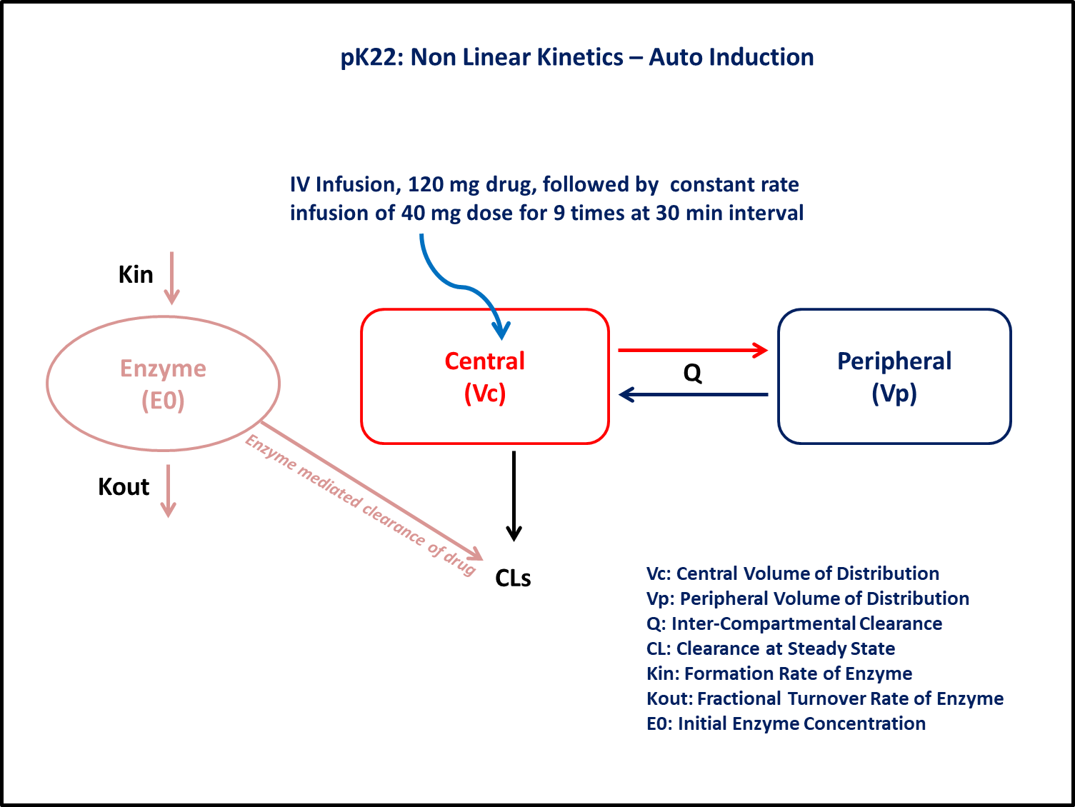
1 Background
- Structural model - Two compartment Model for drug and one compartment model for enzyme
- Route of administration - IV Infusion
- Dosage Regimen - 120 mg of IV infusion at a constant rate of 1 hour followed by 9 more doses of 40 mg for 30 minutes duration at the interval of 8 hours
- Number of Subjects - 1
2 Learning Outcome
This model gives an understanding of drug pharmacokinetics and enzyme autoinduction simultaneously after repeated IV infusion.
3 Objectives
In this tutorial, you will learn how to build a two compartment model for a drug and a one compartment model for an enzyme and simulate from the model.
4 Libraries
Call the necessary libraries to get started.
5 Model
In this two compartment model, we administer repeated doses of IV infusions to a single subject.
pk_22 = @model begin
    @metadata begin
        desc = "Autoinduction Model"
        timeu = u"hr"
    end

    @param begin
        """
        Clearance at Steady State (L/hr)
        """
        tvcls ∈ RealDomain(lower = 0)
        """
        Central Volume of Distribution (L)
        """
        tvvc ∈ RealDomain(lower = 0)
        """
        Peripheral Volume of Distribution (L)
        """
        tvvp ∈ RealDomain(lower = 0)
        """
        Distribution Clearance (L/hr)
        """
        tvq ∈ RealDomain(lower = 0)
        """
        Input Rate Constant for Enzyme (hr⁻¹)
        """
        tvkin ∈ RealDomain(lower = 0)
        """
        Output Rate Constant for Enzyme (hr⁻¹)
        """
        tvkout ∈ RealDomain(lower = 0)
        """
        Initial Enzyme Concentration
        """
        tvE0 ∈ RealDomain(lower = 0)
        Ω ∈ PDiagDomain(7)
        """
        Proportional RUV
        """
        σ²_prop ∈ RealDomain(lower = 0)
    end

    @random begin
        η ~ MvNormal(Ω)
    end

    @pre begin
        Cls = tvcls * exp(η[1])
        Vc = tvvc * exp(η[2])
        Vp = tvvp * exp(η[3])
        Q = tvq * exp(η[4])
        Kin = tvkin * exp(η[5])
        Kout = tvkout * exp(η[6])
        E0 = tvE0 * exp(η[7])
    end

    @init begin
        Enzyme = (Kin / Kout) + E0
    end

    @dynamics begin
        Central' =
            -(Cls / Vc) * Central * Enzyme + (Q / Vp) * Peripheral - (Q / Vc) * Central
        Peripheral' = (Q / Vc) * Central - (Q / Vp) * Peripheral
        Enzyme' = Kin * (E0 + Central / Vc) - Kout * Enzyme
    end

    @derived begin
        cp = @. Central / Vc
        """
        Observed Concentration (mcg/L)
        """
        dv ~ ProportionalNormal.(cp, sqrt(σ²_prop))
    end
end
┌ Warning: Variable `cp` is defined in the `@derived` block using `=` and hence `cp` is not used for model fitting but only returned when simulating: │ If `cp` is a random variable, it must be defined in the `@derived` block using `~`; │ if `cp` should be returned when simulating, it should be defined in the `@observed` block using `=`; │ if `cp` is an intermediate quantity that should not be returned when simulating, it should be defined using `:=`. └ @ Pumas ~/run/_work/PumasTutorials.jl/PumasTutorials.jl/custom_julia_depot/packages/Pumas/GZeMg/src/dsl/model_macro.jl:2351
PumasModel
  Parameters: tvcls, tvvc, tvvp, tvq, tvkin, tvkout, tvE0, Ω, σ²_prop
  Random effects: η
  Covariates:
  Dynamical system variables: Central, Peripheral, Enzyme
  Dynamical system type: Nonlinear ODE
  Derived: cp, dv
  Observed: cp, dv
6 Parameters
Parameters are provided for the simulation. Note that tv represents the typical value for parameters.
tvcls- Typical Value Clearance at Steady State (L/hr)tvvc- Typical Value Central Volume of Distribution (L)tvvp- Typical Value Peripheral Volume of Distribution (L)tvq- Typical Value Distribution Clearance (L/hr)tvkin- Input Rate Constant for Enzyme (hr⁻¹)tvkout- Output Rate Constant for Enzyme (hr⁻¹)tvE0- Initial Enzyme ConcentrationΩ- Between Subject Variabilityσ- Residual errors
param = (
    tvcls = 0.04,
    tvvc = 150.453,
    tvvp = 54.0607,
    tvq = 97.8034,
    tvkin = 0.0238896,
    tvkout = 0.0238896,
    tvE0 = 132.864,
    Ω = Diagonal([0.04, 0.04, 0.04, 0.04, 0.04, 0.04, 0.04]),
    σ²_prop = 0.005,
)
7 Dosage Regimen
Dosage Regimen - 120 mg of IV infusion at a constant rate of 1 hour, followed by 9 more doses of 40 mg for 30 minutes duration at an interval of 8 hours
ev1 = DosageRegimen(
    [120000, 40000],
    time = [0, 8],
    duration = [1, 0.5],
    cmt = [1, 1],
    addl = [0, 8],
    ii = [0, 8],
)
2×10 DataFrame
| Row | time | cmt | amt | evid | ii | addl | rate | duration | ss | route |
|---|---|---|---|---|---|---|---|---|---|---|
| Float64 | Int64 | Float64 | Int8 | Float64 | Int64 | Float64 | Float64 | Int8 | NCA.Route | |
| 1 | 0.0 | 1 | 120000.0 | 1 | 0.0 | 0 | 120000.0 | 1.0 | 0 | NullRoute |
| 2 | 8.0 | 1 | 40000.0 | 1 | 8.0 | 8 | 80000.0 | 0.5 | 0 | NullRoute |
sub1 = Subject(id = 1, events = ev1)Subject
ID: 1
Events: 108 Simulation
Let’s simulate for plasma concentration with the specific observation time points after IV.
Random.seed!(123)The random effects are zero’ed out since we are simulating means
zfx = zero_randeffs(pk_22, sub1, param)(η = [0.0, 0.0, 0.0, 0.0, 0.0, 0.0, 0.0],)sim_sub1 = simobs(pk_22, sub1, param, zfx, obstimes = 0.00:0.01:96)SimulatedObservations
Simulated variables: cp, dv
Time: 0.0:0.01:96.09 Visualization
@chain DataFrame(sim_sub1) begin
    dropmissing(:cp)
    data(_) *
    mapping(:time => "Time (hour)", :cp => "PK22 Concentrations (μg/mL)") *
    visual(Lines, linewidth = 4)
    draw(; axis = (; xticks = 0:10:100), figure = (; fontsize = 22))
end
10 Population simulation
par = (
    tvcls = 0.04,
    tvvc = 150.453,
    tvvp = 54.0607,
    tvq = 97.8034,
    tvkin = 0.0238896,
    tvkout = 0.0238896,
    tvE0 = 132.864,
    Ω = Diagonal([0.0425, 0.0312, 0.0264, 0.0429, 0.0110, 0.0156, 0.0289]),
    σ²_prop = 0.00140536,
)
ev1 = DosageRegimen(
    [120000, 40000],
    time = [0, 8],
    duration = [1, 0.5],
    cmt = [1, 1],
    addl = [0, 8],
    ii = [0, 8],
)
pop = map(i -> Subject(id = i, events = ev1), 1:50)
Random.seed!(1234)
pop_sim = simobs(
    pk_22,
    pop,
    par,
    obstimes = [
        0.25,
        0.5,
        1,
        1.25,
        1.5,
        3,
        5,
        7,
        7.75,
        8.5,
        15.75,
        16.5,
        23.99,
        24.5,
        31.75,
        32.5,
        39.75,
        40.5,
        47.99,
        48.5,
        55.75,
        56.5,
        63.75,
        64.5,
        72,
        72.25,
        72.5,
        72.75,
        73,
        73.5,
        74.5,
        76.5,
        78.5,
        80.5,
        84.5,
        90.5,
        96,
    ],
);

df_sim = DataFrame(pop_sim)
#CSV.write("pk_22.csv", df_sim)