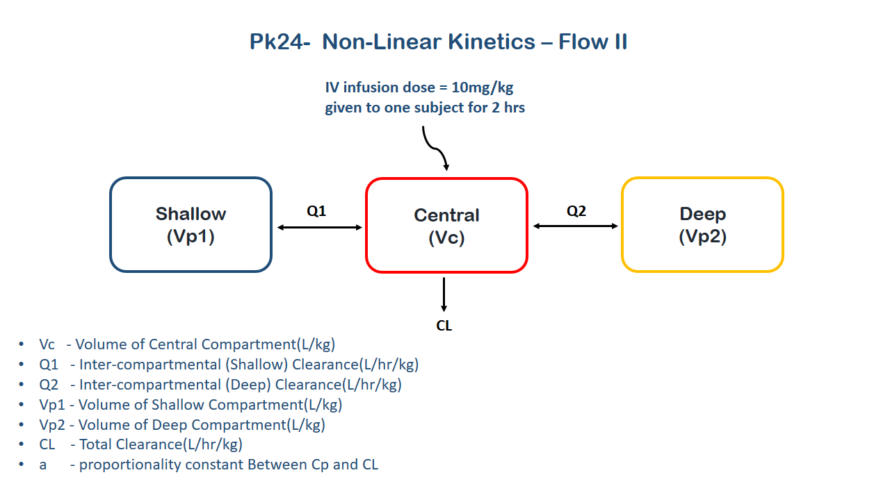
PK24 - Non-linear Kinetics - Flow II

1 Background

• Structural model - Multi-compartment (three) model with concentration dependent clearance
• Route of administration - IV infusion
• Dosage Regimen - One IV infusion dose of 10 mg/kg given for 2 hours.
• Number of Subjects - 1

PK24 Graphic Model

2 Learning Outcomes

This exercise explains a multi-compartment model following concentration dependent clearance.

3 Objectives

In this tutorial, you will learn:

• To build a multi-compartment model with concentration dependent clearance.
• To simulate the data for one subject given an IV infusion for 2 hours.

4 Libraries

Call the necessary libraries to get started.

using Random
using Pumas
using PumasUtilities
using AlgebraOfGraphics
using CairoMakie
using CSV
using DataFramesMeta
using Dates

5 Model

This model contains three compartments (Central, shallow and deep) and the clearance is dependent on the change in plasma concentration due to the drug, which is known to reduce cardiac output and hepatic blood flow with an increase in plasma concentration. The change in clearance can be accounted by the equation: \(CL= CLo-A(Central/Vc)\) where \(A\) is proportionality constant between \(CL\) and \(C\)

pk_24 = @model begin
    @metadata begin
        desc = "Three Compartment Model"
        timeu = u"hr"
    end

    @param begin
        """
        Volume of Central Compartment(L/kg)
        """
        tvvc ∈ RealDomain(lower = 0)
        """
        Clearance(L/hr/kg)
        """
        tvclo ∈ RealDomain(lower = 0)
        """
        Inter-compartmental (Shallow) Clearance(L/hr/kg)
        """
        tvq1 ∈ RealDomain(lower = 0)
        """
        Inter-compartmental (Deep) Clearance(L/hr/kg)
        """
        tvq2 ∈ RealDomain(lower = 0)
        """
        Volume of Shallow Compartment(L/kg)
        """
        tvvp1 ∈ RealDomain(lower = 0)
        """
        Volume of Deep Compartment(L/kg)
        """
        tvvp2 ∈ RealDomain(lower = 0)
        """
        Proportionality constant Between Cp and CL(L2/hr/μg/kg)
        """
        tva ∈ RealDomain(lower = 0)
        Ω ∈ PDiagDomain(7)
        σ_prop ∈ RealDomain(lower = 0)
    end

    @random begin
        η ~ MvNormal(Ω)
    end

    @pre begin
        Vc = tvvc * exp(η[1])
        CLo = tvclo * exp(η[2])
        Q1 = tvq1 * exp(η[3])
        Q2 = tvq2 * exp(η[4])
        Vp1 = tvvp1 * exp(η[5])
        Vp2 = tvvp2 * exp(η[6])
        A = 1000 * tva * exp(η[7])
    end

    @dynamics begin
        Central' =
            -(CLo - (A * (Central / Vc))) * (Central / Vc) - Q1 * (Central / Vc) +
            Q1 * (Shallow / Vp1) - Q2 * (Central / Vc) + Q2 * (Deep / Vp2)
        Shallow' = Q1 * (Central / Vc) - Q1 * (Shallow / Vp1)
        Deep' = Q2 * (Central / Vc) - Q2 * (Deep / Vp2)
    end

    @derived begin
        cp = @. 1000 * Central / Vc
        """
        Observed Concentration (μg/L)
        """
        dv ~ @. Normal(cp, sqrt(cp^2 * σ_prop))
    end
end

PumasModel
  Parameters: tvvc, tvclo, tvq1, tvq2, tvvp1, tvvp2, tva, Ω, σ_prop
  Random effects: η
  Covariates: 
  Dynamical system variables: Central, Shallow, Deep
  Dynamical system type: Nonlinear ODE
  Derived: cp, dv
  Observed: cp, dv

6 Parameters

The parameters are as given below. Note that tv represents the typical value for parameters.

• Vc - Volume of Central Compartment (L/kg)
• CLo - Clearance (L/hr/kg)
• Q1 - Inter-compartmental (Shallow) Clearance (L/hr/kg)
• Q2 - Inter-compartmental (Deep) Clearance (L/hr/kg)
• Vp1 - Volume of Shallow Compartment (L/kg)
• Vp2 - Volume of Deep Compartment (L/kg)
• A - proportionality constant Between Cp and CL (L2/hr/μg/kg)
• Ω - Between Subject Variability
• σ - Residual error (for plasma concentration)

param = (
    tvvc = 0.68,
    tvclo = 6.61,
    tvq1 = 5.94,
    tvq2 = 0.93,
    tvvp1 = 1.77,
    tvvp2 = 3.20,
    tva = 0.0025,
    Ω = Diagonal([0.04, 0.04, 0.04, 0.04, 0.04, 0.04, 0.04]),
    σ_prop = 0.004,
)

7 Dosage Regimen

Build the dosage regimen for one subject given an IV infusion of 10 mg/kg for 2 hours.

DR = DosageRegimen(10, time = 0, cmt = 1, duration = 2)

1×10 DataFrame

Row	time	cmt	amt	evid	ii	addl	rate	duration	ss	route
	Float64	Int64	Float64	Int8	Float64	Int64	Float64	Float64	Int8	NCA.Route
1	0.0	1	10.0	1	0.0	0	5.0	2.0	0	NullRoute

s1 = Subject(id = 1, events = DR)

Subject
  ID: 1
  Events: 2

8 Simulation

The random effects are zero’ed out since we are simulating means

zfx = zero_randeffs(pk_24, s1, param)

(η = [0.0, 0.0, 0.0, 0.0, 0.0, 0.0, 0.0],)

To simulate the data with specific data points.

sim_sub1 = simobs(pk_24, s1, param, zfx, obstimes = 0.1:0.01:8)

SimulatedObservations
  Simulated variables: cp, dv
  Time: 0.1:0.01:8.0

9 Visualization

@chain DataFrame(sim_sub1) begin
    dropmissing(:cp)
    data(_) *
    mapping(:time => "Time (hour)", :cp => "PK24 Concentrations (μg/mL)") *
    visual(Lines, linewidth = 4)
    draw(; axis = (; xticks = 0:2:8), figure = (; fontsize = 22))
end

10 Population simulation

parameters = (
    tvvc = 0.68,
    tvclo = 6.61,
    tvq1 = 5.94,
    tvq2 = 0.93,
    tvvp1 = 1.77,
    tvvp2 = 3.20,
    tva = 0.0025,
    Ω = Diagonal([0.02, 0.0, 0.02, 0.04, 0.02, 0.02, 0.0]),
    σ_prop = 0.039,
)

DR = DosageRegimen(10, time = 0, cmt = 1, duration = 2)
pop = map(i -> Subject(id = i, events = DR), 1:45)

Random.seed!(1234)

ss = simobs(
    pk_24,
    pop,
    parameters,
    obstimes = [
        0.25,
        0.5,
        0.75,
        1.05,
        1.25,
        1.49,
        1.75,
        1.99,
        2.16,
        2.35,
        2.4,
        2.65,
        2.81,
        2.95,
        3.11,
        3.56,
        4.15,
        6,
        7,
    ],
)

df_sim = DataFrame(ss)
#CSV.write("pk_24.csv", df_sim)