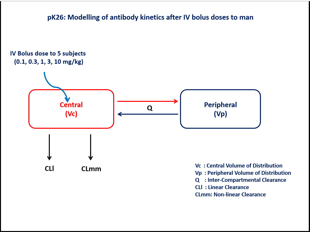
PK26 - Target mediated drug disposition

1 Background

Structural model - Two compartment model with parallel linear and non-linear elimination
Route of administration - IV bolus (Single dose)
Dosage Regimen - 0.1 mg/kg, 0.3 mg/kg, 1 mg/kg, 3 mg/kg, and 10 mg/kg
Number of Subjects - 5

2 Learning Outcomes

To understand the antibody kinetics with linear and nonlinear elimination after an IV bolus dose in man.

3 Objectives

To build a two compartment model with parallel linear and non-linear elimination to understand the antibody kinetics.
To simulate 5 subjects after a single dose IV bolus administration

4 Libraries

Call the necessary libraries to get started.

using Random
using Pumas
using PumasUtilities
using AlgebraOfGraphics
using CairoMakie
using CSV
using DataFramesMeta
using Dates

5 Model

A two compartment model with parallel linear and non-linear elimination

pk_26 = @model begin
    @metadata begin
        desc = "Parallel Linear and Non-linear Elimination Model"
        timeu = u"hr"
    end

    @param begin
        """
        Maximum rate of Metabolism(mg/hr/kg)
        """
        tvvmax ∈ RealDomain(lower = 0)
        """
        Michaelis constant (mg/L/kg)
        """
        tvkm ∈ RealDomain(lower = 0)
        """
        Volume of Peripheral Compartment(L/kg)
        """
        tvvp ∈ RealDomain(lower = 0)
        """
        Volume of Central Compartment(L/kg)
        """
        tvvc ∈ RealDomain(lower = 0)
        """
        Inter-compartmental Clearance(L/hr/kg)
        """
        tvq ∈ RealDomain(lower = 0)
        """
        Linear Clearance(L/hr/kg)
        """
        tvcll ∈ RealDomain(lower = 0)
        Ω ∈ PDiagDomain(6)
        """
        Proportional RUV
        """
        σ²_prop ∈ RealDomain(lower = 0)
    end

    @random begin
        η ~ MvNormal(Ω)
    end

    @pre begin
        Vmax = tvvmax * exp(η[1])
        Km = tvkm * exp(η[2])
        Vp = tvvp * exp(η[3])
        Vc = tvvc * exp(η[4])
        Q = tvq * exp(η[5])
        CLl = tvcll * exp(η[6]) # Linear clearance
        # CLmm       = Vmax/(Km+C)     Non-linear clearance
    end

    @dynamics begin
        Central' =
            -(Vmax / (Km + (Central / Vc))) * (Central / Vc) - CLl * (Central / Vc) -
            (Q / Vc) * Central + (Q / Vp) * Peripheral
        Peripheral' = (Q / Vc) * Central - (Q / Vp) * Peripheral
    end

    @derived begin
        cp = @. Central / Vc
        """
        Observed Concentration (mg/L)
        """
        dv ~ @. Normal(cp, sqrt(cp^2 * σ²_prop))
    end
end

PumasModel
  Parameters: tvvmax, tvkm, tvvp, tvvc, tvq, tvcll, Ω, σ²_prop
  Random effects: η
  Covariates: 
  Dynamical system variables: Central, Peripheral
  Dynamical system type: Nonlinear ODE
  Derived: cp, dv
  Observed: cp, dv

6 Parameters

The parameters are as given below. Note that tv represents the typical value for parameters.

Vmax - Maximum rate of metabolism (mg/hr/kg)
Km - Michaelis constant (mg/L/kg)
Vp - Volume of Peripheral Compartment (L/kg)
Vc - Volume of Central Compartment (L/kg)
Q - Inter-compartmental Clearance (L/hr/kg)
CLl - Linear Clearance (L/hr/kg)
Ω - Between Subject Variability
σ²_prop - Residual error

param = (
    tvvmax = 0.0338,
    tvkm = 0.0760,
    tvvp = 0.0293,
    tvvc = 0.0729,
    tvq = 0.0070,
    tvcll = 0.0069,
    Ω = Diagonal([0.04, 0.04, 0.04, 0.04, 0.04, 0.04]),
    σ²_prop = 0.04,
)

7 Dosage Regimen

5 subjects received an IV bolus dose of 0.1, 0.3, 1, 3 and 10 mg/kg respectively at time=0

DR1 = DosageRegimen(0.1, time = 0)

1×10 DataFrame

Row	time	cmt	amt	evid	ii	addl	rate	duration	ss	route
	Float64	Int64	Float64	Int8	Float64	Int64	Float64	Float64	Int8	NCA.Route
1	0.0	1	0.1	1	0.0	0	0.0	0.0	0	NullRoute

s1 = Subject(id = "0.1 mg/kg", events = DR1, time = 0.1:0.01:1.5)

Subject
  ID: 0.1 mg/kg
  Events: 1

DR2 = DosageRegimen(0.3, time = 0)

1×10 DataFrame

Row	time	cmt	amt	evid	ii	addl	rate	duration	ss	route
	Float64	Int64	Float64	Int8	Float64	Int64	Float64	Float64	Int8	NCA.Route
1	0.0	1	0.3	1	0.0	0	0.0	0.0	0	NullRoute

s2 = Subject(id = "0.3 mg/kg", events = DR2, time = 0.1:0.01:7)

Subject
  ID: 0.3 mg/kg
  Events: 1

DR3 = DosageRegimen(1, time = 0)

1×10 DataFrame

Row	time	cmt	amt	evid	ii	addl	rate	duration	ss	route
	Float64	Int64	Float64	Int8	Float64	Int64	Float64	Float64	Int8	NCA.Route
1	0.0	1	1.0	1	0.0	0	0.0	0.0	0	NullRoute

s3 = Subject(id = "1 mg/kg", events = DR3, time = 0.1:0.1:21)

Subject
  ID: 1 mg/kg
  Events: 1

DR4 = DosageRegimen(3, time = 0)

1×10 DataFrame

Row	time	cmt	amt	evid	ii	addl	rate	duration	ss	route
	Float64	Int64	Float64	Int8	Float64	Int64	Float64	Float64	Int8	NCA.Route
1	0.0	1	3.0	1	0.0	0	0.0	0.0	0	NullRoute

s4 = Subject(id = "3 mg/kg", events = DR4, time = 0.1:0.1:30)

Subject
  ID: 3 mg/kg
  Events: 1

DR5 = DosageRegimen(10, time = 0)

1×10 DataFrame

Row	time	cmt	amt	evid	ii	addl	rate	duration	ss	route
	Float64	Int64	Float64	Int8	Float64	Int64	Float64	Float64	Int8	NCA.Route
1	0.0	1	10.0	1	0.0	0	0.0	0.0	0	NullRoute

s5 = Subject(id = "10 mg/kg", events = DR5, time = 0.1:0.1:43)

Subject
  ID: 10 mg/kg
  Events: 1

pop = [s1, s2, s3, s4, s5]

Population
  Subjects: 5
  Observations:

A more succinct way of generating the pop above across the 5 subjects is given below

doses = [0.1, 0.3, 1, 3, 10]
samp_times = [0.1:0.01:1.5, 0.1:0.01:7, 0.1:0.1:21, 0.1:0.1:30, 0.1:0.1:43]
pop = map(zip(doses, samp_times)) do (d, times)
    Subject(id = string(d, " mg/kg"), events = DosageRegimen(d, time = 0), time = times)
end

Population
  Subjects: 5
  Observations:

8 Simulation

To simulate plasma concentration data for 5 subjects with specific obstimes.

Random.seed!(123)

The random effects are zero’ed out since we are simulating means

zfx = zero_randeffs(pk_26, pop, param)

5-element Vector{NamedTuple{(:η,), Tuple{Vector{Float64}}}}:
 (η = [0.0, 0.0, 0.0, 0.0, 0.0, 0.0],)
 (η = [0.0, 0.0, 0.0, 0.0, 0.0, 0.0],)
 (η = [0.0, 0.0, 0.0, 0.0, 0.0, 0.0],)
 (η = [0.0, 0.0, 0.0, 0.0, 0.0, 0.0],)
 (η = [0.0, 0.0, 0.0, 0.0, 0.0, 0.0],)

sim = simobs(pk_26, pop, param, zfx)

Simulated population (Vector{<:Subject})
  Simulated subjects: 5
  Simulated variables: cp, dv

9 Visualization

@chain DataFrame(sim) begin
    dropmissing(:cp)
    data(_) *
    mapping(
        :time => "Time (days)",
        :cp => "PK26 Concentrations (mg/L)",
        color = :id => nonnumeric => "Doses",
    ) *
    visual(Lines, linewidth = 4)
    draw(;
        axis = (
            yscale = log10,
            yticks = map(i -> 10.0^i, -2:2),
            ytickformat = i -> (@. string(round(i; digits = 1))),
            xticks = 0:10:40,
        ),
        figure = (;
            fontsize = 22,
            legend = (;
                linewidth = 6,
                position = :bottom,
                tellwidth = true,
                tellheight = true,
                width = Auto(),
            ),
        ),
    )
end

10 Population simulation

par = (
    tvvmax = 0.0338,
    tvkm = 0.0760,
    tvvp = 0.0293,
    tvvc = 0.0729,
    tvq = 0.0070,
    tvcll = 0.0069,
    Ω = Diagonal([0.04, 0.03, 0.03, 0.02, 0.04, 0.04]),
    σ²_prop = 0.04,
)

DR1 = DosageRegimen(0.1, time = 0)
DR2 = DosageRegimen(0.3, time = 0)
DR3 = DosageRegimen(1, time = 0)
DR4 = DosageRegimen(3, time = 0)
DR5 = DosageRegimen(10, time = 0)

pop1 = map(i -> Subject(id = i, events = DR1), 1:45)
pop2 = map(i -> Subject(id = i, events = DR2), 46:90)
pop3 = map(i -> Subject(id = i, events = DR3), 91:135)
pop4 = map(i -> Subject(id = i, events = DR4), 136:180)
pop5 = map(i -> Subject(id = i, events = DR5), 181:225)

pop = vcat(pop1, pop2, pop3, pop4, pop5)

Random.seed!(314)
sim_pop1 = simobs(pk_26, pop1, par, obstimes = [0.07, 0.15, 0.33, 0.43, 0.96, 1.2])
sim_pop2 = simobs(
    pk_26,
    pop2,
    par,
    obstimes = [0.23, 0.33, 0.51, 1.18, 1.75, 2.2, 3.06, 3.5, 4, 4.5, 5, 5.5, 6.89],
)
sim_pop3 = simobs(
    pk_26,
    pop3,
    par,
    obstimes = [0.2, 0.4, 1.2, 3.2, 4.5, 6, 7.1, 9, 10, 11, 12, 13, 14.3, 21],
)
sim_pop4 = simobs(
    pk_26,
    pop4,
    par,
    obstimes = [
        0.4,
        0.5,
        0.6,
        1.1,
        3.2,
        5,
        7.1,
        9,
        10,
        12,
        14.2,
        15,
        16,
        17,
        19,
        20.9,
        22,
        24,
        25,
        26,
        27,
        27.5,
        28.1,
    ],
)
sim_pop5 = simobs(
    pk_26,
    pop5,
    par,
    obstimes = [
        0.2,
        0.5,
        1.2,
        2,
        3.2,
        5,
        7.1,
        9,
        12,
        14.1,
        16,
        18,
        20,
        21.1,
        22,
        24,
        25,
        26.5,
        28.1,
        30,
        32,
        34,
        36,
        38,
        40,
        42.1,
    ],
)

populationsimulation = vcat(sim_pop1, sim_pop2, sim_pop3, sim_pop4, sim_pop5)
sim_plot(populationsimulation)

df_pop = DataFrame(populationsimulation)
#CSV.write("pk_26.csv", df_pop)