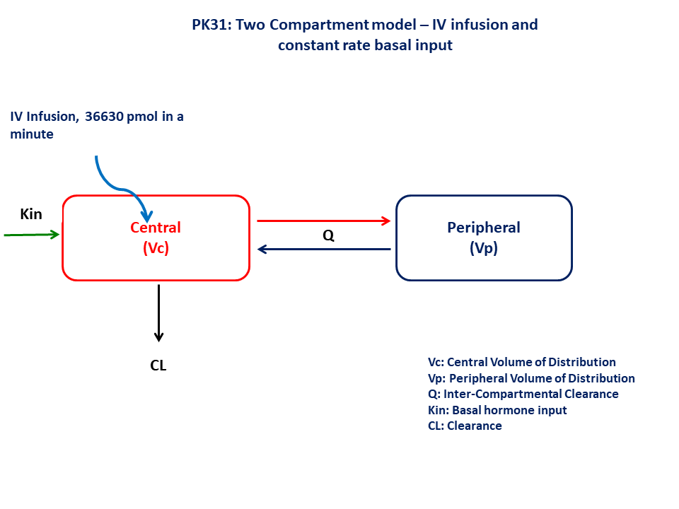
PK31 - Turnover II - Intravenous Dosing of Hormone

1 Background

• Structural model - Two compartment with additional input for basal hormone synthesis in the central compartment
• Route of administration - IV infusion (1 minute)
• Dosage Regimen - 36,630 pmol
• Number of Subjects - 1

PK31 Graphic Model

2 Learning Outcome

In this model, you will learn how to build a two compartment model with additional input for basal hormone level. This model will help to simulate the plasma concentration profile after IV administration, considering basal hormone input.

3 Objectives

• To analyze the intravenous datasets with parallel turnover
• To write a multi-compartment model in terms of differential equations

4 Libraries

Call the necessary libraries to get start.

using Random
using Pumas
using PumasUtilities
using CairoMakie
using AlgebraOfGraphics
using CSV
using DataFramesMeta
using Dates

5 Model

In this one compartment model, we administer an IV infusion dose to the central compartment.

pk_31 = @model begin
    @metadata begin
        desc = "Two Compartment Model"
        timeu = u"hr"
    end

    @param begin
        """
        Basal hormonal input (pmol/hr)
        """
        tvkin ∈ RealDomain(lower = 0)
        """
        Central Volume of Distribution (L)
        """
        tvvc ∈ RealDomain(lower = 0)
        """
        Clearance (L/hr)
        """
        tvcl ∈ RealDomain(lower = 0)
        """
        Intercompartmental Clearance (L/hr)
        """
        tvq ∈ RealDomain(lower = 0)
        """
        Peripheral Volume of Distribution (L)
        """
        tvvp ∈ RealDomain(lower = 0)
        Ω ∈ PDiagDomain(5)
        """
        Proportional RUV
        """
        σ²_prop ∈ RealDomain(lower = 0)

    end

    @random begin
        η ~ MvNormal(Ω)
    end

    @pre begin
        Kin = tvkin * exp(η[1])
        Vc = tvvc * exp(η[2])
        Cl = tvcl * exp(η[3])
        Q = tvq * exp(η[4])
        Vp = tvvp * exp(η[5])
    end

    @dynamics begin
        Central' = Kin - (Cl / Vc) * Central - (Q / Vc) * Central + (Q / Vp) * Peripheral
        Peripheral' = (Q / Vc) * Central - (Q / Vp) * Peripheral
    end

    @derived begin
        cp = @. Central / Vc
        """
        Observed Concentration (pmol/L)
        """
        dv ~ @. Normal(cp, sqrt(cp^2 * σ²_prop))
    end
end

PumasModel
  Parameters: tvkin, tvvc, tvcl, tvq, tvvp, Ω, σ²_prop
  Random effects: η
  Covariates:
  Dynamical system variables: Central, Peripheral
  Dynamical system type: Matrix exponential
  Derived: cp, dv
  Observed: cp, dv

6 Parameters

The parameters are as given below. Note that tv represents the typical value for parameters.

• Kin - Basal hormonal input (pmol/hr)
• Vc - Central Volume of Distribution (L)
• Cl - Clearance (L/hr)
• Q - Intercompartmental Clearance (L/hr)
• Vp - Peripheral Volume of Distribution (L)
• Ω - Between Subject Variability,
• σ - Residual error

param = (
    tvkin = 1531.87,
    tvvc = 8.8455,
    tvcl = 76.5987,
    tvq = 56.8775,
    tvvp = 58.8033,
    Ω = Diagonal([0.04, 0.04, 0.04, 0.04, 0.04]),
    σ²_prop = 0.015,
)

7 Dosage Regimen

A single dose of 36630 pmol is given as an IV Infusion

ev1 = DosageRegimen(36630, time = 0, cmt = 1, duration = 0.0166)

1×10 DataFrame

Row	time	cmt	amt	evid	ii	addl	rate	duration	ss	route
	Float64	Int64	Float64	Int8	Float64	Int64	Float64	Float64	Int8	NCA.Route
1	0.0	1	36630.0	1	0.0	0	2.20663e6	0.0166	0	NullRoute

sub1 = Subject(id = 1, events = ev1)

Subject
  ID: 1
  Events: 1

8 Simulation

Simulate the plasma concentration profile

Random.seed!(123)

The random effects are zero’ed out since we are simulating a single subject

zfx = zero_randeffs(pk_31, sub1, param)

(η = [0.0, 0.0, 0.0, 0.0, 0.0],)

sim_sub1 = simobs(pk_31, sub1, param, zfx, obstimes = 0.01:0.0001:32)

SimulatedObservations
  Simulated variables: cp, dv
  Time: 0.01:0.0001:32.0

9 Visualization

@chain DataFrame(sim_sub1) begin
    dropmissing(:cp)
    data(_) *
    mapping(:time => "Time (hours)", :cp => "Concentration (pmol/L)") *
    visual(Lines; linewidth = 4)
    draw(;
        figure = (; fontsize = 22),
        axis = (;
            yscale = log10,
            ytickformat = i -> (@. string(round(i; digits = 1))),
            xticks = 0:5:35,
        ),
    )
end

10 Population simulation

par = (
    tvkin = 1531.87,
    tvvc = 8.8455,
    tvcl = 76.5987,
    tvq = 56.8775,
    tvvp = 58.8033,
    Ω = Diagonal([0.09, 0.0125, 0.0225, 0.04, 0.0365]),
    σ²_prop = 0.0612144,
)

ev1 = DosageRegimen(36630, time = 0, cmt = 1, duration = 0.0166)
pop = map(i -> Subject(id = i, events = ev1), 1:85)

sim_pop = simobs(
    pk_31,
    pop,
    par,
    obstimes = [
        0.0167,
        0.1167,
        0.167,
        0.25,
        0.583,
        0.833,
        1.083,
        1.583,
        2.083,
        4.083,
        8.083,
        12,
        23.5,
        24.25,
        26.75,
        32,
    ],
)

df_sim = DataFrame(sim_pop)
#CSV.write("pk_31.csv", df_sim)