using Pumas
using PumasUtilities
using Random
using CairoMakie
using AlgebraOfGraphics
using CSV
using DataFramesMeta
PK32 - Turnover III - Non-linear Disposition
1 Learning Outcomes
In this tutorial, we will learn to simulate data for multiple infusions of an endogenous compound with non-linear disposition.
2 Objectives
In this exercise, you will learn how to:
- Build a one compartment model for an endogenous compound with non-linear disposition
- Use final parameter estimates and design a multiple infusion dosage regimen
- Simulate and plot a single subject with predefined time points.
3 Background
Before constructing a model, it is important to establish the process the model will follow and a scenario for the simulation.
Below is the scenario for this tutorial:
- Structural model - One compartment with zero order input and non linear elimination
- Route of administration - IV infusion
- Dosage Regimen - Multiple intravenous infusions (three sets of rapid IV infusions followed by a slow IV infusion)
- Number of Subjects - 1
This diagram describes how such an administered dose will be handled, which facilitates building the model. 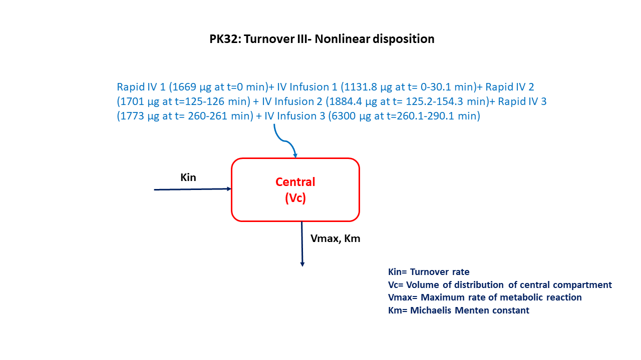
4 Libraries
Call the required libraries to get started.
5 Model
One compartment model for an endogenous compound with non-linear disposition.
pk_32 = @model begin
    @metadata begin
        desc = "Non-linear Elimination Model"
        timeu = u"minute"
    end

    @param begin
        """
        Volume of Central Compartment (L)
        """
        tvvc ∈ RealDomain(lower = 0)
        """
        Maximum metabolic capacity (μg/min)
        """
        tvvmax ∈ RealDomain(lower = 0)
        """
        Michaelis-Menten constant (μg/L)
        """
        tvkm ∈ RealDomain(lower = 0)
        """
        Rate of synthesis (μg/min)
        """
        tvkin ∈ RealDomain(lower = 0)
        """
        Proportional RUV
        """
        σ²_prop ∈ RealDomain(lower = 0)
    end

    @pre begin
        Vc = tvvc
        Vmax = tvvmax
        Km = tvkm
        Kin = tvkin
        #CL      = Vmax/(Km+(Central/Vc))
    end

    @init begin
        Central = Kin / ((Vmax / Km) / Vc)
    end

    @dynamics begin
        Central' = Kin - (Vmax / (Km + Central / Vc)) * (Central / Vc)
    end

    @derived begin
        cp = @. Central / Vc
        """
        Observed Concentration (μg/L)
        """
        dv ~ ProportionalNormal.(cp, sqrt(σ²_prop))
    end
end
┌ Warning: Variable `cp` is defined in the `@derived` block using `=` and hence `cp` is not used for model fitting but only returned when simulating: │ If `cp` is a random variable, it must be defined in the `@derived` block using `~`; │ if `cp` should be returned when simulating, it should be defined in the `@observed` block using `=`; │ if `cp` is an intermediate quantity that should not be returned when simulating, it should be defined using `:=`. └ @ Pumas ~/run/_work/PumasTutorials.jl/PumasTutorials.jl/custom_julia_depot/packages/Pumas/GZeMg/src/dsl/model_macro.jl:2351
PumasModel
  Parameters: tvvc, tvvmax, tvkm, tvkin, σ²_prop
  Random effects:
  Covariates:
  Dynamical system variables: Central
  Dynamical system type: Nonlinear ODE
  Derived: cp, dv
  Observed: cp, dv
6 Parameters
The parameters are as given below.
Vc- Volume of Central Compartment (L)Vmax- Maximum metabolic capacity (μg/min)Km- Michaelis-menten constant (μg/L)Kin- Rate of synthesis, Turnover rate (μg/min)σ- Residual error
These are the initial estimates we will be using in this model exercise. Note that tv represents the typical value for parameters.
param =
    (; tvvc = 5.94952, tvvmax = 361.502, tvkm = 507.873, tvkin = 14.9684, σ²_prop = 0.05)
7 Dosage Regimen
DosageRegimen - Three sets of rapid intravenous infusions followed by a slow intravenous infusion are defined and coded as follows:
- IV bolus of 1669 μg (Time = 0 min) followed by IV infusion of 1131.8 μg (Time = 0-30.1 min)
- IV infusion of 1701 μg (Time = 0-30.1 min) followed by IV infusion of 1884.4 μg (Time = 125.2-154.3 min)
- IV infusion of 1773 μg (Time = 260-261 min) followed by IV infusion of 6300 μg (Time = 260.1-290.1 min)
IVinfRapid = DosageRegimen(
    [1669, 1701, 1733];
    time = [0, 125, 260],
    cmt = [1, 1, 1],
    duration = [0, 1, 1],
)
3×10 DataFrame
| Row | time | cmt | amt | evid | ii | addl | rate | duration | ss | route |
|---|---|---|---|---|---|---|---|---|---|---|
| Float64 | Int64 | Float64 | Int8 | Float64 | Int64 | Float64 | Float64 | Int8 | NCA.Route | |
| 1 | 0.0 | 1 | 1669.0 | 1 | 0.0 | 0 | 0.0 | 0.0 | 0 | NullRoute |
| 2 | 125.0 | 1 | 1701.0 | 1 | 0.0 | 0 | 1701.0 | 1.0 | 0 | NullRoute |
| 3 | 260.0 | 1 | 1733.0 | 1 | 0.0 | 0 | 1733.0 | 1.0 | 0 | NullRoute |
IVinfSlow = DosageRegimen(
    [1131.8, 1884.4, 6300];
    time = [0, 125.2, 260.1],
    cmt = [1, 1, 1],
    duration = [30.1, 29.1, 30],
)
3×10 DataFrame
| Row | time | cmt | amt | evid | ii | addl | rate | duration | ss | route |
|---|---|---|---|---|---|---|---|---|---|---|
| Float64 | Int64 | Float64 | Int8 | Float64 | Int64 | Float64 | Float64 | Int8 | NCA.Route | |
| 1 | 0.0 | 1 | 1131.8 | 1 | 0.0 | 0 | 37.6013 | 30.1 | 0 | NullRoute |
| 2 | 125.2 | 1 | 1884.4 | 1 | 0.0 | 0 | 64.756 | 29.1 | 0 | NullRoute |
| 3 | 260.1 | 1 | 6300.0 | 1 | 0.0 | 0 | 210.0 | 30.0 | 0 | NullRoute |
This is how to establish the dosing regimen:
DR = DosageRegimen(IVinfRapid, IVinfSlow)6×10 DataFrame
| Row | time | cmt | amt | evid | ii | addl | rate | duration | ss | route |
|---|---|---|---|---|---|---|---|---|---|---|
| Float64 | Int64 | Float64 | Int8 | Float64 | Int64 | Float64 | Float64 | Int8 | NCA.Route | |
| 1 | 0.0 | 1 | 1669.0 | 1 | 0.0 | 0 | 0.0 | 0.0 | 0 | NullRoute |
| 2 | 0.0 | 1 | 1131.8 | 1 | 0.0 | 0 | 37.6013 | 30.1 | 0 | NullRoute |
| 3 | 125.0 | 1 | 1701.0 | 1 | 0.0 | 0 | 1701.0 | 1.0 | 0 | NullRoute |
| 4 | 125.2 | 1 | 1884.4 | 1 | 0.0 | 0 | 64.756 | 29.1 | 0 | NullRoute |
| 5 | 260.0 | 1 | 1733.0 | 1 | 0.0 | 0 | 1733.0 | 1.0 | 0 | NullRoute |
| 6 | 260.1 | 1 | 6300.0 | 1 | 0.0 | 0 | 210.0 | 30.0 | 0 | NullRoute |
This is how to create the single subject undergoing the dosing regimen above.
sub1 = Subject(; id = 1, events = DR)Subject
ID: 1
Events: 68 Simulation
To simulate plasma concentration for a single subject with the specific observation time points for a given dosage regimen DR.
NoteRandom.seed!()
The Random.seed! function is included here for purposes of reproducibility of the simulation in this tutorial. Specification of a seed value would not be required in a Pumas workflow that is estimating model parameters.
Random.seed!(123)sim = simobs(pk_32, sub1, param, obstimes = 0:0.01:450)SimulatedObservations
Simulated variables: cp, dv
Time: 0.0:0.01:450.09 Visualization
From the plot, the multiple infusions can be witnessed through the presence of multiple peaks at different time points.
@chain DataFrame(sim) begin
    dropmissing(:cp)
    data(_) *
    mapping(:time => "Time (min)", :cp => "Concentration (μg/L)") *
    visual(Lines; linewidth = 4)
    draw(; figure = (; fontsize = 22), axis = (; xticks = 0:50:450))
end
10 Population Simulation
This block updates the parameters of the model to increase intersubject variability in parameters and defines timepoints for the prediction of concentrations. The results are written to a CSV file.
par = (tvvc = 5.94952, tvvmax = 361.502, tvkm = 507.873, tvkin = 14.9684, σ = 0.05)

IVinfRapid = DosageRegimen(
    [1669, 1701, 1733];
    time = [0, 125, 260],
    cmt = [1, 1, 1],
    duration = [0, 1, 1],
)
IVinfSlow = DosageRegimen(
    [1131.8, 1884.4, 6300];
    time = [0, 125.2, 260.1],
    cmt = [1, 1, 1],
    duration = [30.1, 29.1, 30],
)
DR = DosageRegimen([IVinfRapid, IVinfSlow])
pop = map(i -> Subject(id = i, events = DR), 1:85)

Random.seed!(1234)
sim_pop = simobs(
    pk_32,
    pop,
    param,
    obstimes = [
        0,
        2.23,
        4.2,
        6.05,
        8.03,
        10,
        15,
        20,
        25,
        30,
        32,
        34.1,
        36.1,
        38.1,
        40.1,
        42,
        45.1,
        50,
        55,
        60,
        70,
        80,
        90.2,
        100,
        110,
        120,
        122.8,
        127,
        129,
        131,
        133,
        135,
        140,
        145.1,
        150,
        154,
        156,
        158,
        160,
        162,
        164,
        166,
        169,
        174,
        179,
        186.8,
        218,
        249,
        250,
        255,
        262.2,
        264.2,
        265.9,
        268,
        270,
        275.1,
        280,
        285,
        290,
        292,
        294.1,
        296.2,
        298.1,
        300,
        302.4,
        305.2,
        310.1,
        315.2,
        320,
        350.1,
        380,
        400,
        450,
    ],
)

df_sim = DataFrame(sim_pop)
#CSV.write("pk_32.csv", df_sim)
NoteSaving the Simulation Results
With the CSV.write function, you can input the name of the DataFrame (df_sim) and the file name of your choice (pk_32.csv) to save the file to your local directory or repository.
11 Conclusion
Constructing a model for multiple infusions with non-linear disposition involves:
- understanding the process of how the drug is passed through the system,
- translating processes into ODEs using Pumas, and
- simulating the model in a single patient for evaluation.