using Random
using Pumas
using PumasUtilities
using CairoMakie
using AlgebraOfGraphics
using CSV
using DataFramesMeta
PK33 - Transdermal input and kinetics
1 Learning Outcome
To understand the kinetics of a given drug using transdermal input following 2 different input rates
2 Objectives
To build a one compartment model with zero-order input and to understand its function using a transdermal delivery system
3 Background
Before constructing a model, it is important to establish the process the model will follow and a scenario for the simulation.
Below is the scenario for this tutorial:
- Structural model - One compartment linear elimination with zero-order input
- Route of administration - Transdermal
- Dosage Regimen - 15,890 μg per patch. The patch was applied for 16 hours over 5 consecutive days
- Number of Subjects - 1
This diagram describes how such an administered dose will be handled, which facilitates building the model. 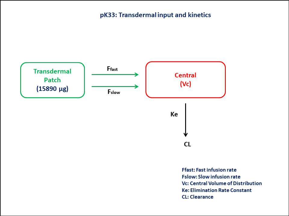
4 Libraries
Call the required libraries to get started.
5 Model
This is a one compartment model with zero-order input following transdermal drug administration.
pk_33 = @model begin
    @metadata begin
        desc = "One Compartment Model"
        timeu = u"hr"
    end

    @param begin
        """
        Clearance (L/hr)
        """
        tvcl ∈ RealDomain(lower = 0)
        """
        Volume of Central Compartment (L)
        """
        tvvc ∈ RealDomain(lower = 0)
        """
        Dose of slow infusion (μg)
        """
        tvdslow ∈ RealDomain(lower = 0)
        """
        Duration of fast release (hr)
        """
        tvtfast ∈ RealDomain(lower = 0)
        """
        Duration of slow release (hr)
        """
        tvtslow ∈ RealDomain(lower = 0)
        Ω ∈ PDiagDomain(5)
        """
        Proportional RUV
        """
        σ²_prop ∈ RealDomain(lower = 0)
        """
        Additional RUV
        """
        σ_add ∈ RealDomain(lower = 0)
    end

    @random begin
        η ~ MvNormal(Ω)
    end

    @pre begin
        Cl = tvcl * exp(η[1])
        Vc = tvvc * exp(η[2])
        Dose_slow = tvdslow * exp(η[3])
        Tfast = tvtfast * exp(η[4])
        Tslow = tvtslow * exp(η[5])
        Ffast = (t <= Tfast) * (15890 - Dose_slow) / Tfast
        Fslow = (t <= Tslow) * Dose_slow / Tslow
    end

    @init begin
        Central = 2 * Vc
    end

    @dynamics begin
        Central' = Ffast + Fslow - (Cl / Vc) * Central
    end

    @derived begin
        cp = @. Central / Vc
        """
        Observed Concentration (μg/L)
        """
        dv ~ CombinedNormal.(cp, σ_add, sqrt(σ²_prop))
    end
end
┌ Warning: Variable `cp` is defined in the `@derived` block using `=` and hence `cp` is not used for model fitting but only returned when simulating: │ If `cp` is a random variable, it must be defined in the `@derived` block using `~`; │ if `cp` should be returned when simulating, it should be defined in the `@observed` block using `=`; │ if `cp` is an intermediate quantity that should not be returned when simulating, it should be defined using `:=`. └ @ Pumas ~/run/_work/PumasTutorials.jl/PumasTutorials.jl/custom_julia_depot/packages/Pumas/GZeMg/src/dsl/model_macro.jl:2351
PumasModel
  Parameters: tvcl, tvvc, tvdslow, tvtfast, tvtslow, Ω, σ²_prop, σ_add
  Random effects: η
  Covariates:
  Dynamical system variables: Central
  Dynamical system type: Nonlinear ODE
  Derived: cp, dv
  Observed: cp, dv
6 Parameters
These are the initial estimates we will be using in this model exercise. Note that tv represents the typical value for parameters.
CL- Clearance (L/hr),Vc- Volume of Central Compartment (L)Dslow- Dose of slow infusion (μg)Tfast- Duration of fast release (hr)Tslow- Duration of slow release (hr)Ω- Between Subject Variabilityσ- Residual error
param = (;
    tvcl = 79.8725,
    tvvc = 239.94,
    tvdslow = 11184.3,
    tvtfast = 7.54449,
    tvtslow = 19.3211,
    Ω = Diagonal([0.01, 0.01, 0.01, 0.01, 0.01]),
    σ²_prop = 0.005,
    σ_add = 0.01,
)
7 Dosage Regimen
- 15,890 μg per patch.
- The patch is applied for 16 hours, for 5 consecutive days
- The patch releases the drug at two different rate processes, fast and slow, simultaneously over a period of 6 and 18 hours respectively.
sub1 = Subject(; id = 1)Subject
ID: 18 Simulation
Since the model is created and the initial parameters are specified, one should evaluate the model. Simulating with a single subject is one way to address this.
NoteRandom.seed!()
The Random.seed! function is included here for purposes of reproducibility of the simulation in this tutorial. Specification of a seed value would not be required in a Pumas workflow that is estimating model parameters.
Random.seed!(123)sim_sub1 = simobs(pk_33, sub1, param, obstimes = 0:0.1:24)SimulatedObservations
Simulated variables: cp, dv
Time: 0.0:0.1:24.09 Visualization
@chain DataFrame(sim_sub1) begin
    dropmissing(:cp)
    data(_) *
    mapping(:time => "Time (hours)", :cp => "Concentration (μg/L)") *
    visual(Lines; linewidth = 4)
    draw(; figure = (; fontsize = 22), axis = (; xticks = 0:5:25))
end
10 Population Simulation
This block updates the parameters of the model to increase intersubject variability in parameters and defines timepoints for the prediction of concentrations. The results are written to a CSV file.
par = (
    tvcl = 79.8725,
    tvvc = 239.94,
    tvdslow = 11184.3,
    tvtfast = 7.54449,
    tvtslow = 19.3211,
    Ω = Diagonal([0.012, 0.024, 0.012, 0.01, 0.012]),
    σ²_prop = 0.008,
    σ_add = 0.01,
)

ev1 = DosageRegimen(15890; time = 0, cmt = 1)
pop = map(i -> Subject(id = i, events = ev1), 1:24)

Random.seed!(1234)
sim_pop = simobs(
    pk_33,
    pop,
    par,
    obstimes = [0, 0.5, 1, 2, 3, 4, 6, 8, 10, 12, 14, 16, 17, 18, 21, 23.37],
)
df_sim = DataFrame(sim_pop)

#CSV.write("pk_33.csv", df_sim)
NoteSaving the Simulation Results
With the CSV.write function, you can input the name of the DataFrame (df_sim) and the file name of your choice (pk_33.csv) to save the file to your local directory or repository.
11 Conclusion
Constructing a transdermal one-compartment model with zero-order input involves:
- understanding the process of how the drug is passed through the system,
- translating processes into ODEs using Pumas,
- preparing the data using Pumas data wrangling functionality, and
- simulating the model in a single patient for evaluation.