PK34 - Reversible metabolism

1 Learning Outcome

In this tutorial, you will learn how to simulate

kinetics of a drug that exhibits reversible metabolism, and
data for two IV-Infusion regimens with different rates of infusions.

2 Objectives

In this exercise, you will learn how to simulate an IV-infusion two compartment model and the kinetics of reversible metabolism.

3 Background

Before constructing a model, it is important to establish the process the model will follow and a scenario for the simulation.

Below is the scenario for this tutorial:

Structural model - Two compartment model
Route of administration - IV-infusion (with an infusion pump)
Dosage Regimen - 100 mg/m² of Cisplatin for 1 hour at time=0 considering a patient with 1.7 m²
Number of Subjects - 1

This diagram describes how such an administered dose will be handled, which facilitates building the model. 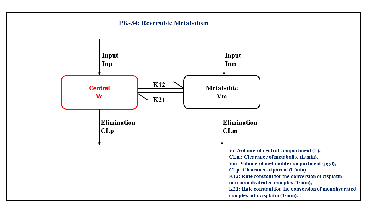PK34 Model Graphic

4 Assumptions to Consider

A fraction of the dose (2.3%) is present as the monohydrated complex in the infusion solution.
There is a reversible reaction between cisplatin (p) and its monohydrated complex (m).
The input rate can be split into a cisplatin infusion rate (Inp) and a monohydrate infusion rate (Inm).

5 Libraries

Call the required libraries to get started.

using Pumas
using PumasUtilities
using Random
using CairoMakie
using AlgebraOfGraphics
using CSV
using DataFramesMeta

6 Model - Microconstant Model

In this two compartment model, we administer the mentioned dose in the Central compartment and the Metabolite compartment at time = 0. K12 and K21 are rate constants for the conversion of cisplatin into monohydrated complex and the monohydrated complex into cisplatin, respectively.

pk_34 = @model begin
    @metadata begin
        desc = "Microconstant Model"
        timeu = u"minute"
    end

    @param begin
        """
        Volume of Central Compartment (L)
        """
        tvvc ∈ RealDomain(lower = 0)
        """
        Clearance of metabolite (L/min)
        """
        tvclm ∈ RealDomain(lower = 0)
        """
        Volume of Metabolite Compartment (μg/L)
        """
        tvvm ∈ RealDomain(lower = 0)
        """
        Clearance of parent (L/min)
        """
        tvclp ∈ RealDomain(lower = 0)
        tvk12 ∈ RealDomain(lower = 0)
        tvk21 ∈ RealDomain(lower = 0)
        Ω ∈ PDiagDomain(6)
        """
        Proportional RUV
        """
        σ²_prop ∈ RealDomain(lower = 0)
    end

    @random begin
        η ~ MvNormal(Ω)
    end

    @pre begin
        Vc = tvvc * exp(η[1])
        CLm = tvclm * exp(η[2])
        Vm = tvvm * exp(η[3])
        CLp = tvclp * exp(η[4])
        K12 = tvk12 * exp(η[5])
        K21 = tvk21 * exp(η[6])
    end

    @dynamics begin
        Central' = -(CLp / Vc) * Central - K12 * Central + K21 * Metabolite * Vc / Vm
        Metabolite' =
            -(CLm / Vm) * Metabolite - K21 * Metabolite + K12 * Central * Vm / Vc
    end

    @derived begin
        cp = @. Central / Vc
        """
        Observed Concentration - Cisplatin (μg/ml)
        """
        dv_cp ~ @. Normal(cp, sqrt(cp^2 * σ²_prop))
        met = @. Metabolite / Vm
        """
        Observed Concentration - Metabolite (μg/ml)
        """
        dv_met ~ @. Normal(met, sqrt(cp^2 * σ²_prop))
    end
end

PumasModel
  Parameters: tvvc, tvclm, tvvm, tvclp, tvk12, tvk21, Ω, σ²_prop
  Random effects: η
  Covariates: 
  Dynamical system variables: Central, Metabolite
  Dynamical system type: Matrix exponential
  Derived: cp, dv_cp, met, dv_met
  Observed: cp, dv_cp, met, dv_met

7 Parameters

Parameters provided for simulation are as below.

Vc - Volume of central compartment (L)
CLm - Clearance of metabolite (L/min)
Vm - Volume of metabolite compartment (μg/L)
CLp - Clearance of parent (L/min)
K12 - Rate constant for the conversion of cisplatin into monohydrated complex (min⁻¹)
K21 - Rate constant for the conversion of monohydrated complex into cisplatin (min⁻¹)
Ω - Between Subject Variability
σ - Residual error

These are the initial estimates we will be using in this model exercise. Note that tv represents the typical value for parameters.

param = (;
    tvvc = 14.1175,
    tvclm = 0.00832616,
    tvvm = 2.96699,
    tvclp = 0.445716,
    tvk12 = 0.00021865,
    tvk21 = 0.021313,
    Ω = Diagonal([0.01, 0.01, 0.01, 0.01, 0.01, 0.01]),
    σ²_prop = 0.001,
)

8 Dosage Regimen

To start the simulation process, the dosing regimen specified in the background section must be developed first prior to running a simulation.

The dosage regimen is specified as:

Cisplatin Infusion - A total dose of 170 mg (100 mg/m² * 1.7 m²) split as Cisplatin 166.09 and Monohydrate 3.91.
Monohydrate Infusion - A total dose of 10 mg/L is given as Monohydrate

This is how to establish the dosing regimen:

ev1 = DosageRegimen([166.09, 3.91]; time = 0, cmt = [1, 2], duration = [60, 60])

2×10 DataFrame

Row	time	cmt	amt	evid	ii	addl	rate	duration	ss	route
	Float64	Int64	Float64	Int8	Float64	Int64	Float64	Float64	Int8	NCA.Route
1	0.0	1	166.09	1	0.0	0	2.76817	60.0	0	NullRoute
2	0.0	2	3.91	1	0.0	0	0.0651667	60.0	0	NullRoute

This is how to create the single subject undergoing the dosing regimen above.

sub1 = Subject(id = "Cisplatin (Inf-Cisplatin)", events = ev1, time = 20:0.1:180)

Subject
  ID: Cisplatin (Inf-Cisplatin)
  Events: 4

The above two steps will be repeated to create the Monohydrate infusion group.

ev2 = DosageRegimen(10; time = 0, cmt = 2, duration = 2)

1×10 DataFrame

Row	time	cmt	amt	evid	ii	addl	rate	duration	ss	route
	Float64	Int64	Float64	Int8	Float64	Int64	Float64	Float64	Int8	NCA.Route
1	0.0	2	10.0	1	0.0	0	5.0	2.0	0	NullRoute

sub2 = Subject(id = "Monohydrate (Inf-Cisplatin)", events = ev2, time = 5:0.1:180)

Subject
  ID: Monohydrate (Inf-Cisplatin)
  Events: 2

Creating the population:

pop2_sub = [sub1, sub2]

Population
  Subjects: 2
  Observations:

9 Simulation

We will simulate the plasma concentration at the pre-specified time points.

Random.seed!()

The Random.seed! function is included here for purposes of reproducibility of the simulation in this tutorial. Specification of a seed value would not be required in a Pumas workflow that is estimating model parameters.

Random.seed!(123)

sim_sub1 = simobs(pk_34, pop2_sub, param)

Simulated population (Vector{<:Subject})
  Simulated subjects: 2
  Simulated variables: cp, dv_cp, met, dv_met

10 Visualization

From the plots, we can see the plasma and metabolite concentrations for both infusion groups.

We will first convert the simulation results into a DataFrame to facilitate plotting.

df_plot = DataFrame(sim_sub1)

This plot is for the parent drug:

@chain df_plot begin
    dropmissing(:cp)
    data(_) *
    mapping(
        :time => "Time (hours)",
        :cp => "Parent concentration (μg/mL)";
        color = :id => "Infusion group",
    ) *
    visual(Lines; linewidth = 4)
    draw(;
        figure = (; fontsize = 22),
        axis = (; xticks = 0:20:180),
        legend = (; position = :bottom),
    )
end

This plot is for the metabolite:

@chain df_plot begin
    dropmissing(:met)
    data(_) *
    mapping(
        :time => "Time (hours)",
        :met => "Metabolite concentration (μg/mL)";
        color = :id => "Infusion group",
    ) *
    visual(Lines; linewidth = 4)
    draw(;
        figure = (; fontsize = 22),
        axis = (; xticks = 0:20:180),
        legend = (; position = :bottom),
    )
end

11 Conclusion

In this tutorial, a drug with two IV-Infusion regimens, which exhibits reversible metabolism, was fit to a model. Constructing a model such as this involves:

understanding the process of how the drug and metabolite are passed through the system,
quantitatively explaining non-linear kinetics of elimination, and
simulating the model in a single patient for evaluation.