using PumasUtilities
using Random
using Pumas
using CairoMakie
using AlgebraOfGraphics
using CSV
using DataFramesMeta
using Dates
PK39 - Two compartment linear elimination with zero order absorption model
1 Background
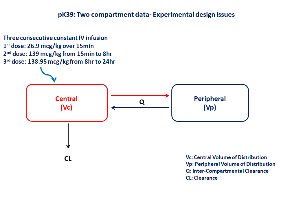
- Structural model - Two compartment linear elimination with zero order absorption
- Route of administration - Three consecutive constant rate IV infusions
- Dosage Regimen - 1st dose: 26.9 mcg/kg over 15 minutes, 2nd dose: 139 mcg/kg from 15 minutes to 8 hours, 3rd dose: 138.95 mcg/kg between 8 and 24 hours
- Number of Subjects - 1
2 Learning Outcome
This exercise demonstrates simulating three consecutive constant rate IV infusions from a two compartment model.
3 Objectives
To build a two-compartment model, simulate the model for a subject given three consecutive constant rate IV infusions, and subsequently perform a simulation for a population.
4 Libraries
Load the necessary libraries.
5 Model definition
Note the expression of the model parameters with helpful comments. The model is expressed with differential equations. Residual variability is a proportional error model.
In this two compartment model, we administer three consecutive IV infusions for a single subject.
pk_39 = @model begin
    @metadata begin
        desc = "Two Compartment Model"
        timeu = u"hr"
    end

    @param begin
        """
        Clearance (L/kg/hr)
        """
        tvcl ∈ RealDomain(lower = 0)
        """
        Volume of Central Compartment (L/kg)
        """
        tvvc ∈ RealDomain(lower = 0)
        """
        Volume of Peripheral Compartment (L/kg)
        """
        tvvp ∈ RealDomain(lower = 0)
        """
        Intercompartmental clearance (L/kg/hr)
        """
        tvq ∈ RealDomain(lower = 0)
        #Ω ∈ PDiagDomain(4)
        Ω_cl ∈ RealDomain(lower = 0.0001)
        Ω_vc ∈ RealDomain(lower = 0.0001)
        Ω_vp ∈ RealDomain(lower = 0.0001)
        Ω_q ∈ RealDomain(lower = 0.0001)
        """
        Proportional RUV
        """
        σ²_prop ∈ RealDomain(lower = 0)
    end

    @random begin
        η_cl ~ Normal(0, sqrt(Ω_cl))
        η_vc ~ Normal(0, sqrt(Ω_vc))
        η_vp ~ Normal(0, sqrt(Ω_vp))
        η_q ~ Normal(0, sqrt(Ω_q))
    end

    @pre begin
        CL = tvcl * exp(η_cl)
        Vc = tvvc * exp(η_vc)
        Vp = tvvp * exp(η_vp)
        Q = tvq * exp(η_q)
    end

    @dynamics begin
        Central' = (Q / Vp) * Peripheral - (Q / Vc) * Central - (CL / Vc) * Central
        Peripheral' = -(Q / Vp) * Peripheral + (Q / Vc) * Central
    end

    @derived begin
        cp = @. Central / Vc
        """
        Observed Concentration (μg/L)
        """
        dv ~ ProportionalNormal.(cp, sqrt(σ²_prop))
    end
end
┌ Warning: Variable `cp` is defined in the `@derived` block using `=` and hence `cp` is not used for model fitting but only returned when simulating: │ If `cp` is a random variable, it must be defined in the `@derived` block using `~`; │ if `cp` should be returned when simulating, it should be defined in the `@observed` block using `=`; │ if `cp` is an intermediate quantity that should not be returned when simulating, it should be defined using `:=`. └ @ Pumas ~/run/_work/PumasTutorials.jl/PumasTutorials.jl/custom_julia_depot/packages/Pumas/GZeMg/src/dsl/model_macro.jl:2351
PumasModel
  Parameters: tvcl, tvvc, tvvp, tvq, Ω_cl, Ω_vc, Ω_vp, Ω_q, σ²_prop
  Random effects: η_cl, η_vc, η_vp, η_q
  Covariates:
  Dynamical system variables: Central, Peripheral
  Dynamical system type: Matrix exponential
  Derived: cp, dv
  Observed: cp, dv
6 Initial Estimates of Model Parameters
The model parameters for simulation are the following. Note that tv represents the typical value for parameters.
Cl- Clearance (L/kg/hr)Vc- Volume of Central Compartment (L/kg)Vp- Volume of Peripheral Compartment (L/kg)Q- Intercompartmental clearance (L/kg/hr)Ω- Between Subject Variabilityσ- Residual error
param = (
    tvcl = 0.417793,
    tvvc = 0.320672,
    tvvp = 2.12265,
    tvq = 0.903188,
    Ω_cl = 0.01,
    Ω_vc = 0.01,
    Ω_vp = 0.01,
    Ω_q = 0.01,
    σ²_prop = 0.005,
)
7 Dosage regimen
Dosage regimen - Single subject receiving three consecutive IV infusions
- 1st dose: 26.9 mcg/kg over 15 minutes
- 2nd dose: 139 mcg/kg from 15 minutes to 8 hours
- 3rd dose: 138.95 mcg/kg between 8 and 24 hours
ev1 = DosageRegimen(
    [26.9, 139, 138.95],
    time = [0, 0.25, 8],
    cmt = 1,
    duration = [0.25, 7.85, 16],
)
3×10 DataFrame
| Row | time | cmt | amt | evid | ii | addl | rate | duration | ss | route |
|---|---|---|---|---|---|---|---|---|---|---|
| Float64 | Int64 | Float64 | Int8 | Float64 | Int64 | Float64 | Float64 | Int8 | NCA.Route | |
| 1 | 0.0 | 1 | 26.9 | 1 | 0.0 | 0 | 107.6 | 0.25 | 0 | NullRoute |
| 2 | 0.25 | 1 | 139.0 | 1 | 0.0 | 0 | 17.707 | 7.85 | 0 | NullRoute |
| 3 | 8.0 | 1 | 138.95 | 1 | 0.0 | 0 | 8.68437 | 16.0 | 0 | NullRoute |
8 Single-individual that receives the defined dose
sub1 = Subject(id = 1, events = ev1)Subject
ID: 1
Events: 39 Single-Subject Simulation
Simulate for plasma concentration with the specific observation time points after IV infusion.
Initialize the random number generator with a seed for reproducibility of the simulation.
Random.seed!(123)Define the timepoints at which concentration values will be simulated.
sim_sub1 = simobs(pk_39, sub1, param, obstimes = 0:0.01:60)SimulatedObservations
Simulated variables: cp, dv
Time: 0.0:0.01:60.010 Visualize Results
@chain DataFrame(sim_sub1) begin
    dropmissing(:cp)
    data(_) *
    mapping(:time => "Time (hours)", :cp => "Concentration (μg/L)") *
    visual(Lines; linewidth = 4)
    draw(; figure = (; fontsize = 22), axis = (; xticks = 0:10:60))
end
11 Population Simulation
We perform a population simulation with 72 participants.
This code demonstrates how to write the simulated concentrations to a comma separated file (.csv).
par = (
    tvcl = 0.417793,
    tvvc = 0.320672,
    tvvp = 2.12265,
    tvq = 0.903188,
    Ω_cl = 0.0123,
    Ω_vc = 0.0625,
    Ω_vp = 0.0154,
    Ω_q = 0.0198,
    σ²_prop = 0.005,
)

ev1 = DosageRegimen(26.9, time = 0, cmt = 1, duration = 0.25)
ev2 = DosageRegimen(139, time = 0.25, cmt = 1, duration = 7.85)
ev3 = DosageRegimen(138.95, time = 8, cmt = 1, duration = 16)
evs = DosageRegimen(ev1, ev2, ev3)
pop = map(i -> Subject(id = i, events = evs), 1:72)

Random.seed!(1234)
sim_pop = simobs(
    pk_39,
    pop,
    par,
    obstimes = [
        0.25,
        0.5,
        1,
        2,
        3,
        6,
        8,
        9,
        10,
        12,
        18,
        21,
        24,
        24.5,
        25,
        26,
        28,
        30,
        32,
        34,
        36,
        42,
        48,
        60,
    ],
)

df_sim = DataFrame(sim_pop)
pkdata_39_sim = DataFrame(sim_pop)

#CSV.write("pk_39_sim.csv", pkdata_39_sim);
12 Conclusion
This tutorial showed how to build a two-compartment linear elimination with zero order absorption model and perform a single subject and a population simulation.