using PumasUtilities
using Random
using Pumas
using CairoMakie
using AlgebraOfGraphics
using CSV
using DataFramesMeta
using Dates
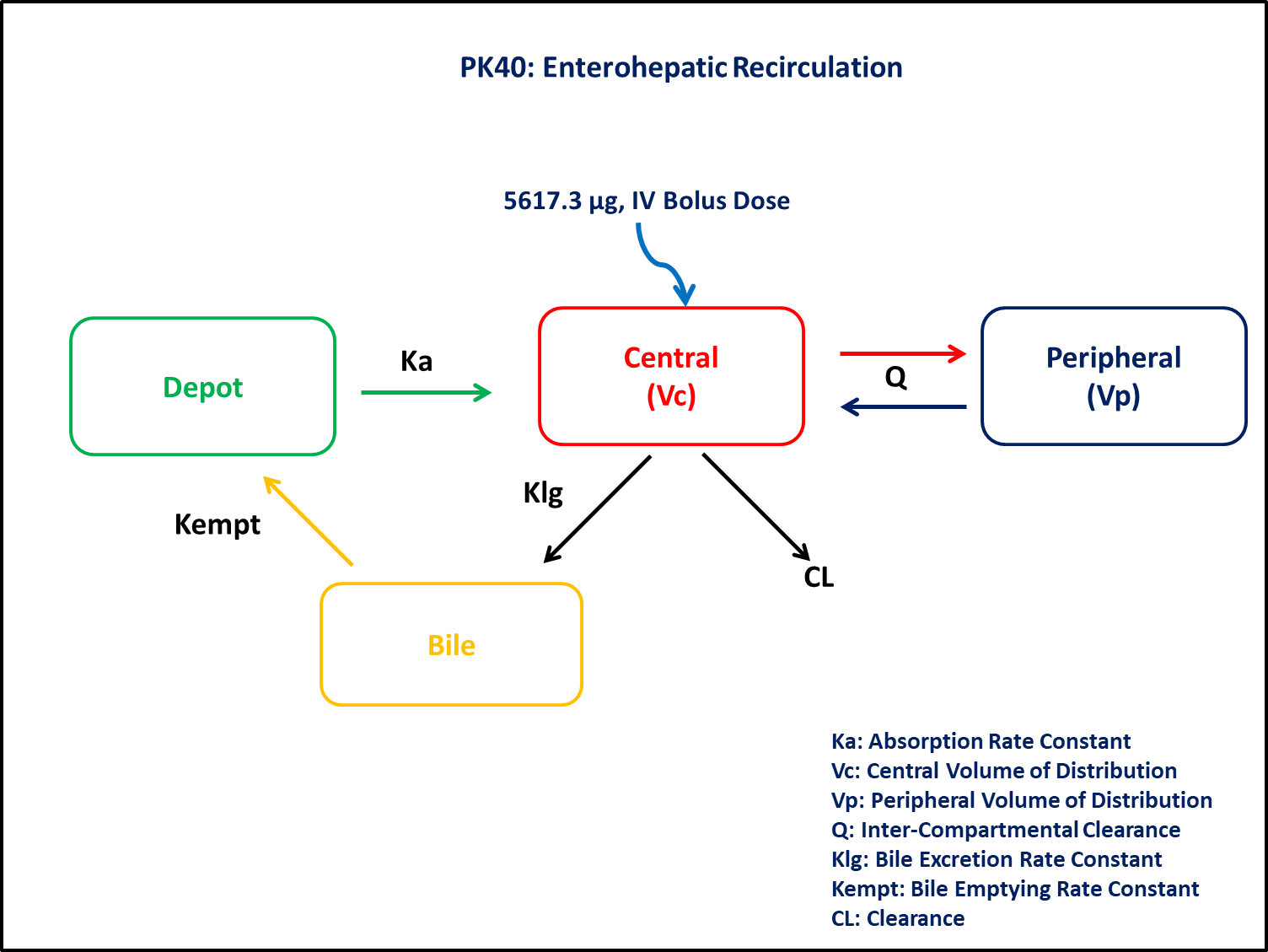
PK40 - Multi-compartment model with Enterohepatic Recirculation after IV administration
1 Background
- Structural model - Enterohepatic Recirculation (EHS)
- Route of administration - IV bolus dose
- Dosage Regimen - 5617.3 μg IV bolus dose was administered and drug plasma concentration was measured for 36 hours
- Number of Subjects - 1
2 Learning Outcome
This exercise demonstrates IV bolus dose kinetics from a multi-compartment model with Enterohepatic Recirculation.
3 Objectives
To build a multi-compartment model with Enterohepatic Recirculation, simulate the model for a single subject given an IV bolus dose and subsequently perform a simulation for a population.
4 Libraries
Load the necessary libraries.
5 Model definition
Note the expression of the model parameters with helpful comments. The model is expressed with differential equations. Residual variability is a proportional error model.
It is a multi-compartment model with Enterohepatic Recirculation
pk_40 = @model begin
    @metadata begin
        desc = "Enterohepatic Recirculation Model"
        timeu = u"hr"
    end

    @param begin
        """
        Clearance (L/hr)
        """
        tvcl ∈ RealDomain(lower = 0)
        """
        Central Volume of Distribution (L)
        """
        tvvc ∈ RealDomain(lower = 0)
        """
        Peripheral Volume of Distribution (L)
        """
        tvvp ∈ RealDomain(lower = 0)
        """
        Intercompartmental Clearance (L/hr)
        """
        tvQ ∈ RealDomain(lower = 0)
        """
        Absorption rate Constant (hr⁻¹)
        """
        tvka ∈ RealDomain(lower = 0)
        """
        Bile Excretion rate constant (hr⁻¹)
        """
        tvklg ∈ RealDomain(lower = 0)
        """
        Bile emptying Interval (hr)
        """
        tvτ ∈ RealDomain(lower = 0)
        Ω ∈ PDiagDomain(7)
        """
        Proportional RUV
        """
        σ²_prop ∈ RealDomain(lower = 0)
    end

    @random begin
        η ~ MvNormal(Ω)
    end

    @pre begin
        Cl = tvcl * exp(η[1])
        Vc = tvvc * exp(η[2])
        Vp = tvvp * exp(η[3])
        Q = tvQ * exp(η[4])
        Ka = tvka * exp(η[5])
        Klg = tvklg * exp(η[6])
        τ = tvτ * exp(η[7])
        Kempt = (t > 10 && t < (10 + τ)) * (1 / τ)
    end

    @dynamics begin
        Central' =
            Ka * Depot - (Cl / Vc) * Central + (Q / Vp) * Peripheral - (Q / Vc) * Central - Klg * Central
        Peripheral' = (Q / Vc) * Central - (Q / Vp) * Peripheral
        Bile' = Klg * Central - Bile * Kempt
        Depot' = Bile * Kempt - Ka * Depot

    end

    @derived begin
        cp = @. Central / Vc
        """
        Observed Concentration (μg/L)
        """
        dv ~ ProportionalNormal.(cp, sqrt(σ²_prop))
    end
end
┌ Warning: Variable `cp` is defined in the `@derived` block using `=` and hence `cp` is not used for model fitting but only returned when simulating: │ If `cp` is a random variable, it must be defined in the `@derived` block using `~`; │ if `cp` should be returned when simulating, it should be defined in the `@observed` block using `=`; │ if `cp` is an intermediate quantity that should not be returned when simulating, it should be defined using `:=`. └ @ Pumas ~/run/_work/PumasTutorials.jl/PumasTutorials.jl/custom_julia_depot/packages/Pumas/GZeMg/src/dsl/model_macro.jl:2351
PumasModel
  Parameters: tvcl, tvvc, tvvp, tvQ, tvka, tvklg, tvτ, Ω, σ²_prop
  Random effects: η
  Covariates:
  Dynamical system variables: Central, Peripheral, Bile, Depot
  Dynamical system type: Nonlinear ODE
  Derived: cp, dv
  Observed: cp, dv
6 Initial Estimates of Model Parameters
The model parameters for simulation are the following. Note that tv represents the typical value for parameters.
tvcl- Clearance (L/hr)tvvc- Central Volume of Distribution (L)tvvp- Peripheral Volume of Distribution (L)tvQ- Intercompartmental Clearance (L/hr)tvka- Absorption rate Constant (hr⁻¹)tvklg- Bile Excretion rate constant (hr⁻¹)tvτ- Typical Value bile emptying Interval (hr)Kempt- Bile Emptying rate constant (hr⁻¹)Ω- Between Subject Variabilityσ- Residual error
param = (
    tvcl = 0.842102,
    tvvc = 12.8201,
    tvvp = 29.0867,
    tvQ = 11.3699,
    tvka = 3.01245,
    tvklg = 0.609319,
    tvτ = 2.79697,
    Ω = Diagonal([0.1, 0.1, 0.1, 0.1, 0.1, 0.1, 0.1]),
    σ²_prop = 0.5,
)
7 Dosage Regimen
A 5617.3 μg IV bolus dose is administered at time 0 and drug plasma concentration was measured for 36 hours
ev1 = DosageRegimen(5617.3, time = 0, cmt = 1)1×10 DataFrame
| Row | time | cmt | amt | evid | ii | addl | rate | duration | ss | route |
|---|---|---|---|---|---|---|---|---|---|---|
| Float64 | Int64 | Float64 | Int8 | Float64 | Int64 | Float64 | Float64 | Int8 | NCA.Route | |
| 1 | 0.0 | 1 | 5617.3 | 1 | 0.0 | 0 | 0.0 | 0.0 | 0 | NullRoute |
8 Single-individual that receives the defined dose
sub1 = Subject(id = 1, events = ev1)Subject
ID: 1
Events: 19 Single-Subject Simulation
Simulate the plasma concentration after IV administration
Initialize the random number generator with a seed for reproducibility of the simulation.
Random.seed!(123)Define the timepoints at which concentration values will be simulated.
sim1 = simobs(pk_40, sub1, param, obstimes = 0:0.1:36)SimulatedObservations
Simulated variables: cp, dv
Time: 0.0:0.1:36.010 Visualize Results
@chain DataFrame(sim1) begin
    dropmissing(:cp)
    data(_) *
    mapping(:time => "Time (hours)", :cp => "Concentration (μg/L)") *
    visual(Lines; linewidth = 4)
    draw(; figure = (; fontsize = 22), axis = (; xticks = 0:5:40))
end
11 Population Simulation
We perform a population simulation with 50 participants.
This code demonstrates how to write the simulated concentrations to a comma separated file (.csv).
par = (
    tvcl = 0.842102,
    tvvc = 12.8201,
    tvvp = 29.0867,
    tvQ = 11.3699,
    tvka = 3.01245,
    tvklg = 0.609319,
    tvτ = 2.79697,
    Ω = Diagonal([0.012, 0.0423, 0.0342, 0.0465, 0.0129, 0.0278, 0.0532]),
    σ²_prop = 0.0677818,
)

ev1 = DosageRegimen(5617.3, time = 0, cmt = 1)
pop = map(i -> Subject(id = i, events = ev1), 1:50)

Random.seed!(1234)
pop_sim = simobs(
    pk_40,
    pop,
    par,
    obstimes = [
        0.03,
        0.083,
        0.15,
        0.17,
        0.33,
        0.5,
        0.67,
        0.83,
        1,
        1.5,
        2,
        4,
        6,
        8,
        10,
        10.5,
        11,
        11.5,
        12,
        12.5,
        13,
        15,
        16,
        17,
        18,
        20,
        24,
        26,
        28,
        30,
        32,
        36,
    ],
)

pkdata_40_sim = DataFrame(pop_sim)
#CSV.write("pk_40_sim.csv", pkdata_40_sim)
12 Conclusion
This tutorial showed how to build a multi-compartment model with Enterohepatic Recirculation and perform a single subject and a population simulation.