PK41 - Multiple Intravenous Infusions: NCA vs Regression

1 Background

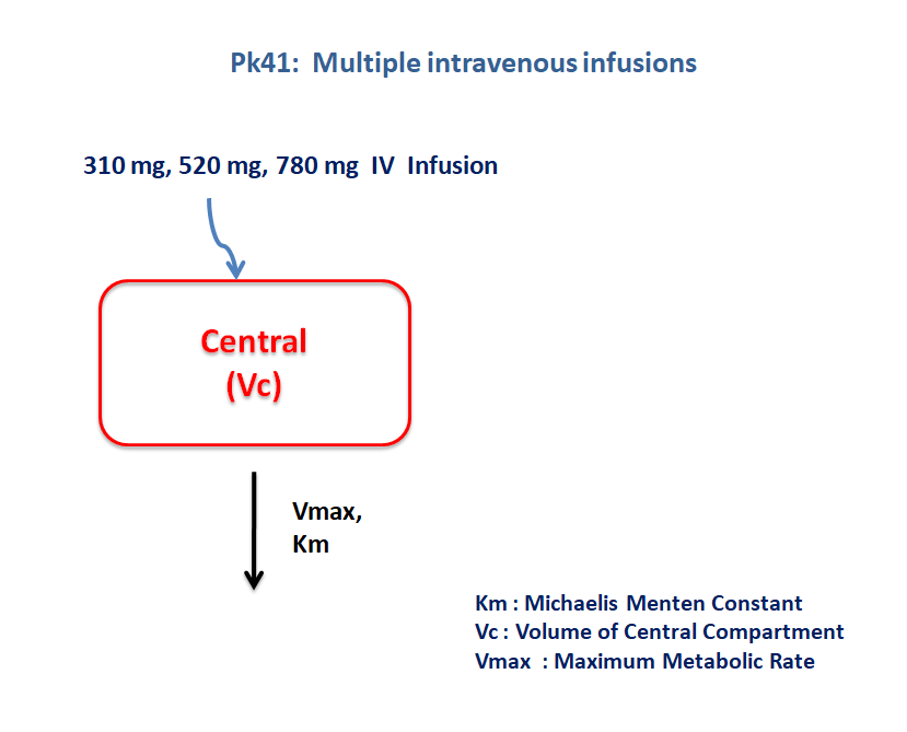
Structural Model - One compartment model with non-linear elimination.
Route of administration - IV infusion
Dosage Regimen - 310 μg, 520 μg, and 780 μg
Number of Subjects - 3

2 Learning Outcome

This is a one compartment model with capacity limited elimination. The concentration time profile was obtained for three subjects administered with three different dosage regimens.

3 Objectives

In this tutorial, you will learn how to build a one compartment model with non-linear elimination.

4 Libraries

Call the necessary libraries to get started.

using Random
using Pumas
using PumasUtilities
using CairoMakie
using AlgebraOfGraphics
using DataFramesMeta
using CSV
using Dates

5 Model

The following model describes the parameters and the differential equation for a one-compartment model with capacity limited elimination

pk_41 = @model begin
    @metadata begin
        desc = "One Compartment Model"
        timeu = u"hr"
    end

    @param begin
        """
        Maximum Metabolic Rate (μg/kg/hr)
        """
        tvvmax ∈ RealDomain(lower = 0)
        """
        Michaelis Menten Constant (μg/kg/L)
        """
        tvkm ∈ RealDomain(lower = 0)
        """
        Volume of Central Compartment (L/kg)
        """
        tvvc ∈ RealDomain(lower = 0)
        Ω ∈ PDiagDomain(3)
        """
        Proportional RUV
        """
        σ²_prop ∈ RealDomain(lower = 0)
    end

    @random begin
        η ~ MvNormal(Ω)
    end

    @pre begin
        Vmax = tvvmax * exp(η[1])
        Km = tvkm * exp(η[2])
        Vc = tvvc * exp(η[3])
    end

    @dynamics begin
        Central' = -(Vmax * (Central / Vc) / (Km + (Central / Vc)))
    end

    @derived begin
        cp = @. Central / Vc
        """
        Observed Concentrations (μg/L)
        """
        dv ~ @. Normal(cp, sqrt(cp^2 * σ²_prop))
    end

    @observed begin
        conc = Central / Vc
        nca := @nca conc
        cl = NCA.cl(nca)
    end
end

PumasModel
  Parameters: tvvmax, tvkm, tvvc, Ω, σ²_prop
  Random effects: η
  Covariates: 
  Dynamical system variables: Central
  Dynamical system type: Nonlinear ODE
  Derived: cp, dv
  Observed: cp, dv, conc, cl

6 Parameters

The parameters are as given below. Note that tv represents the typical value for parameters.

Vmax - Maximum Metabolic Rate (μg/kg/hr)
Km - Michaelis Menten Constant (μg/kg/L)
Vc - Volume of Central compartment (L/kg)

param = (
    tvvmax = 180.311,
    tvkm = 79.8382,
    tvvc = 1.80036,
    Ω = Diagonal([0.04, 0.04, 0.04, 0.04, 0.04]),
    σ²_prop = 0.015,
)

7 Dosage Regimen

All subjects receive an IV infusion over 5 hours with the following doses:

Subject 1 receives a dose of 310 μg
Subject 2 receives a dose of 520 μg
Subject 3 receives a dose of 780 μg

dose = [310, 520, 780]

rate_ind = [62, 104, 156]

ids = ["310 μg.kg-1", "520 μg.kg-1", "780 μg.kg-1"]

ev(x) =
    DosageRegimen(dose[x], cmt = 1, time = 0, rate = rate_ind[x], route = NCA.IVInfusion)

ev (generic function with 1 method)

pop3_sub = map(i -> Subject(id = ids[i], events = ev(i)), 1:length(ids))

Population
  Subjects: 3
  Observations:

8 Simulation

Simulate the plasma concentration of the drug for all the subjects

Random.seed!(123)

The random effects are zero’ed out since we are simulating a single subject

zfx = zero_randeffs(pk_41, pop3_sub, param)

3-element Vector{NamedTuple{(:η,), Tuple{Vector{Float64}}}}:
 (η = [0.0, 0.0, 0.0],)
 (η = [0.0, 0.0, 0.0],)
 (η = [0.0, 0.0, 0.0],)

time_values = 0.1:0.01:10
sim_pop3_sub = simobs(pk_41, pop3_sub, param, zfx, obstimes = time_values)

Simulated population (Vector{<:Subject})
  Simulated subjects: 3
  Simulated variables: cp, dv, conc, cl

9 Visualization

We will build a DataFrame to facilitate plotting

cp_values = [i.observations.cp for i in sim_pop3_sub]
df_subs = [
    DataFrame(:cp => cp_values[i], :id => ids[i], :time => time_values) for
    i in eachindex(ids)
]
df_plot = vcat(df_subs...)

@chain df_plot begin
    dropmissing(:cp)
    data(_) *
    mapping(:time => "Time (hours)", :cp => "Concentration (μg/L)", color = :id => "Dose") *
    visual(Lines; linewidth = 4)
    draw(;
        figure = (; fontsize = 22),
        axis = (;
            xticks = 0:10,
            yscale = log10,
            ytickformat = i -> (@. string(round(i; digits = 1))),
        ),
        legend = (; position = :bottom),
    )
end

df_41 = reduce(vcat, map(sim_pop3_sub) do subj
    subdf = DataFrame(id = subj.subject.id, cl = subj.observations.cl)
end)
@chain df_41 begin
    dropmissing!(:cl)
    unique([:id, :cl])
    data(_) *
    mapping(:id => nonnumeric => "Dose", :cl => "Cl (L/hr/kg)") *
    visual(ScatterLines, linewidth = 4, markersize = 22)
    draw(axis = (; yticks = 0.8:0.2:1.8,), figure = (; fontsize = 22))
end

10 Simulating a Population

par = (
    tvvmax = 180.311,
    tvkm = 79.8382,
    tvvc = 1.80036,
    Ω = Diagonal([0.0462, 0.0628, 0.0156, 0.0321, 0.0126]),
    σ²_prop = 0.0234,
)

ev1 = DosageRegimen(310, cmt = 1, time = 0, rate = 62, route = NCA.IVInfusion)
pop1 = map(i -> Subject(id = i, events = ev1), 1:20)
ev2 = DosageRegimen(520, cmt = 1, time = 0, rate = 104, route = NCA.IVInfusion)
pop2 = map(i -> Subject(id = i, events = ev2), 21:40)
ev3 = DosageRegimen(780, cmt = 1, time = 0, rate = 156, route = NCA.IVInfusion)
pop3 = map(i -> Subject(id = i, events = ev3), 41:60)
pop = [pop1; pop2; pop3]

Random.seed!(1234)
sim_pop = simobs(pk_41, pop, par, obstimes = [0, 0.1, 2, 5, 6, 8, 10])

df_sim = reduce(
    vcat,
    map(sim_pop) do subj
        subdf = DataFrame(
            id = subj.subject.id,
            time = subj.time,
            cp = subj.observations.cp,
            cl = subj.observations.cl,
        )
    end,
);

#CSV.write("pk_41.csv", df_sim)