using PumasUtilities
using Random
using Pumas
using CairoMakie
using AlgebraOfGraphics
using CSV
using DataFramesMeta
using Dates
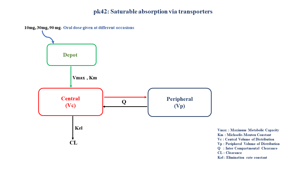
PK42 - Saturable absorption via transporters
1 Background
- Structural model - Multi compartment model with saturable absorption kinetics
- Route of administration - Oral Route
- Dosage Regimen - 10 mg, 30 mg, and 90 mg oral dose given at different occasions
- Number of Subjects - 1
2 Learning Outcomes
This model gives an understanding of non-linear absorption due to saturation of drug transporters at higher doses of drug administered orally.
3 Objectives
To build a multi-compartment model for a drug following saturable absorption kinetics, simulate the model for a single subject given an oral dose at different occasions, and subsequently perform a simulation for a population.
4 Libraries
Load the necessary libraries.
5 Model definition
Note the expression of the model parameters with helpful comments. The model is expressed with differential equations. Residual variability is an additive error model.
In this multi compartment model, a single subject receives oral doses of a compound X on three different occasions, which follows non-linear absorption and linear disposition kinetics.
pk_42 = @model begin
    @metadata begin
        desc = "Non-linear Absorption Model"
        timeu = u"minute"
    end

    @param begin
        """
        Maximum Metabolic Capacity (μg/min)
        """
        tvvmax ∈ RealDomain(lower = 0)
        """
        Michaelis-Menten Constant (μg/L)
        """
        tvkm ∈ RealDomain(lower = 0)
        """
        Volume of Distribution of Central Compartment (L)
        """
        tvvc ∈ RealDomain(lower = 0)
        """
        Volume of Distribution of Peripheral compartment (L)
        """
        tvvp ∈ RealDomain(lower = 0)
        """
        Inter Compartmental Clearance (L/min)
        """
        tvq ∈ RealDomain(lower = 0)
        """
        Clearance (L/min)
        """
        tvcl ∈ RealDomain(lower = 0)
        #Ω ∈ PDiagDomain(6)
        Ω_vmax ∈ RealDomain(lower = 0.0001)
        Ω_km ∈ RealDomain(lower = 0.0001)
        Ω_vc ∈ RealDomain(lower = 0.0001)
        Ω_vp ∈ RealDomain(lower = 0.0001)
        Ω_q ∈ RealDomain(lower = 0.0001)
        Ω_cl ∈ RealDomain(lower = 0.0001)
        """
        Additive RUV
        """
        σ_add ∈ RealDomain(lower = 0)
    end

    @random begin
        η_vmax ~ Normal(0, sqrt(Ω_vmax))
        η_km ~ Normal(0, sqrt(Ω_km))
        η_vc ~ Normal(0, sqrt(Ω_vc))
        η_vp ~ Normal(0, sqrt(Ω_vp))
        η_q ~ Normal(0, sqrt(Ω_q))
        η_cl ~ Normal(0, sqrt(Ω_cl))
    end

    @pre begin
        Vmax = tvvmax * exp(η_vmax)
        Km = tvkm * exp(η_km)
        Vc = tvvc * exp(η_vc)
        Vp = tvvp * exp(η_vp)
        Q = tvq * exp(η_q)
        CL = tvcl * exp(η_cl)
    end

    @vars begin
        VMKM := Vmax / (Km + Depot)
    end

    @dynamics begin
        Depot' = -VMKM * Depot
        Central' =
            VMKM * Depot - CL * (Central / Vc) - (Q / Vc) * Central + (Q / Vp) * Peripheral
        Peripheral' = (Q / Vc) * Central - (Q / Vp) * Peripheral
    end

    @derived begin
        cp = @. Central / Vc
        """
        Observed Concentration (μg/L)
        """
        dv ~ @. Normal(cp, σ_add)
    end
end
┌ Warning: Variable `cp` is defined in the `@derived` block using `=` and hence `cp` is not used for model fitting but only returned when simulating: │ If `cp` is a random variable, it must be defined in the `@derived` block using `~`; │ if `cp` should be returned when simulating, it should be defined in the `@observed` block using `=`; │ if `cp` is an intermediate quantity that should not be returned when simulating, it should be defined using `:=`. └ @ Pumas ~/run/_work/PumasTutorials.jl/PumasTutorials.jl/custom_julia_depot/packages/Pumas/GZeMg/src/dsl/model_macro.jl:2351
PumasModel
  Parameters: tvvmax, tvkm, tvvc, tvvp, tvq, tvcl, Ω_vmax, Ω_km, Ω_vc, Ω_vp, Ω_q, Ω_cl, σ_add
  Random effects: η_vmax, η_km, η_vc, η_vp, η_q, η_cl
  Covariates:
  Dynamical system variables: Depot, Central, Peripheral
  Dynamical system type: Nonlinear ODE
  Derived: cp, dv
  Observed: cp, dv
6 Initial Estimates of Model Parameters
The model parameters for simulation are the following. Note that tv represents the typical value for parameters.
Vmax- Maximum Metabolic Capacity (μg/min)Km- Michaelis-Menten Constant (μg/ml)Vc- Volume of Distribution of the Central Compartment (L)Vp- Volume of Distribution of the Peripheral compartment (L)Q- Inter Compartmental Clearance (L/min)CL- Clearance (L/min)Ω- Between Subject Variabilityσ- Residual Error
param = (
    tvvmax = 982.453,
    tvkm = 9570.63,
    tvvc = 4.66257,
    tvvp = 35,
    tvq = 0.985,
    tvcl = 2.00525,
    Ω_vmax = 0.01,
    Ω_km = 0.01,
    Ω_vc = 0.01,
    Ω_vp = 0.01,
    Ω_q = 0.01,
    Ω_cl = 0.01,
    σ_add = 0.123,
)
7 Dosage Regimen
A single subject received oral dosing of 10, 30, 90 mg on three different occasions
dose_ind = [10000, 30000, 90000]8 Single-individual that receives the defined dose
ids = ["10 mg", "30 mg", "90 mg"]ev(x) = DosageRegimen(dose_ind[x], time = 0, cmt = 1)pop = map(i -> Subject(id = ids[i], events = ev(i)), eachindex(ids))Population
Subjects: 3
Observations: 9 Single-Subject Simulation
Simulate the plasma concentration for a single subject after an oral dose given on three different occasions.
Initialize the random number generator with a seed for reproducibility of the simulation.
Random.seed!(123)Define the timepoints at which concentration values will be simulated.
sim_pop3_sub = simobs(pk_42, pop, param, obstimes = 0.1:0.1:360)Simulated population (Vector{<:Subject})
Simulated subjects: 3
Simulated variables: cp, dv10 Visualize Results
@chain DataFrame(sim_pop3_sub) begin
    dropmissing(:cp)
    data(_) *
    mapping(
        :time => "Time (minutes)",
        :cp => "Concentration (μg/L)";
        color = :id => "Dose",
    ) *
    visual(Lines; linewidth = 4)
    draw(;
        figure = (; fontsize = 22),
        axis = (;
            yscale = log10,
            ytickformat = i -> (@. string(round(i; digits = 1))),
            xticks = 0:50:400,
        ),
        legend = (; position = :bottom),
    )
end
11 Population Simulation
We perform a population simulation with 48 participants, and simulate concentration values for 72 hours following 6 doses administered every 8 hours.
This code demonstrates how to write the simulated concentrations to a comma separated file (.csv).
par = (
    tvvmax = 982.453,
    tvkm = 9570.63,
    tvvc = 4.66257,
    tvvp = 35,
    tvq = 0.985,
    tvcl = 2.00525,
    Ω_vmax = 0.0123,
    Ω_km = 0.0325,
    Ω_vc = 0.062,
    Ω_vp = 0.005,
    Ω_q = 0.004,
    Ω_cl = 0.008,
    σ_add = 0.823,
)

ev1 = DosageRegimen(90000, time = 0, cmt = 1)
pop1 = map(i -> Subject(id = i, events = ev1, covariates = (Dose = "10 mg",)), 1:34)
ev2 = DosageRegimen(30000, time = 0, cmt = 1)
pop2 = map(i -> Subject(id = i, events = ev2, covariates = (Dose = "30 mg",)), 1:34)
ev3 = DosageRegimen(10000, time = 0, cmt = 1)
pop3 = map(i -> Subject(id = i, events = ev3, covariates = (Dose = "90 mg",)), 1:34)
pop = [pop1; pop2; pop3]

Random.seed!(1234)
pop_sim = simobs(
    pk_42,
    pop,
    par,
    obstimes = [
        0.1,
        5,
        10,
        15,
        20,
        25,
        30,
        35,
        40,
        45,
        50,
        55,
        60,
        70,
        75,
        80,
        85,
        90,
        95,
        105,
        110,
        115,
        120,
        150,
        180,
        210,
        240,
        300,
        360,
    ],
)

pkdata_42_sim = DataFrame(pop_sim)
#CSV.write("pk_42_sim.csv", pkdata_42_sim)
12 Conclusion
This tutorial showed how to build a multi compartment model for a drug after saturation and perform a single subject and a population simulation.