using Pumas
using PumasUtilities
using Random
using CairoMakie
using AlgebraOfGraphics
using CSV
using DataFramesMeta
PK43 - Multiple Absorption Routes
1 Learning Outcome
In this exercise, we will be looking at multiple absorption routes and how a model helps in understanding the absorption of sublingually administered doses, partly from the buccal cavity and partly from the gastrointestinal (GI) tract.
2 Objectives
In this model, you will learn how to write a differential equation model for a drug that is partly absorbed from the buccal and partly from the GI and simulate for a single subject.
3 Background
Before constructing a model, it is important to establish the process the model will follow and a scenario for the simulation.
Below is the scenario for this tutorial:
- Structural model - 1 compartment linear elimination with first order absorption
- Route of administration - Sublingual
- Dosage Regimen - 2 mg Sublingual dose
- Number of Subjects - 1
This diagram describes how such an administered dose will be handled, which facilitates building the model. 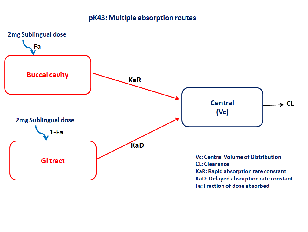
4 Libraries
Call the required libraries to get started.
5 Model
In this one compartment model, we administer the dose sublingually at 2 sites. Both sites are accounted for in the @dosecontrol block, including the lag time from the absorption process occurring physiologically in the GI tract.
pk_43 = @model begin
    @metadata begin
        desc = "Multiple Absorption Model"
        timeu = u"hr"
    end

    @param begin
        """
        Absorption rate constant(rapid from buccal) (hr⁻¹)
        """
        tvkar ∈ RealDomain(lower = 0)
        """
        Absorption rate constant(delayed from GI) (hr⁻¹)
        """
        tvkad ∈ RealDomain(lower = 0)
        """
        Volume of Central Compartment (L)
        """
        tvv ∈ RealDomain(lower = 0)
        """
        Lagtime (hr)
        """
        tvlag ∈ RealDomain(lower = 0)
        """
        Fraction of drug absorbed
        """
        tvfa ∈ RealDomain(lower = 0)
        """
        Elimination rate constant (hr⁻¹)
        """
        tvk ∈ RealDomain(lower = 0)
        Ω ∈ PDiagDomain(4)
        """
        Additive RUV
        """
        σ_add ∈ RealDomain(lower = 0)
    end

    @random begin
        η ~ MvNormal(Ω)
    end

    @pre begin
        KaR = tvkar * exp(η[1])
        KaD = tvkad * exp(η[2])
        V = tvv * exp(η[3])
        K = tvk * exp(η[4])
    end

    @dosecontrol begin
        bioav = (Buccal = tvfa, Gi = 1 - tvfa)
        lags = (Gi = tvlag,)
    end

    @dynamics begin
        Buccal' = -KaR * Buccal
        Gi' = -KaD * Gi
        Central' = KaR * Buccal + KaD * Gi - K * Central
    end

    @derived begin
        cp = @. Central / V
        """
        Observed Concentration (mcg/L)
        """
        dv ~ @. Normal(cp, σ_add)
    end
end
┌ Warning: Variable `cp` is defined in the `@derived` block using `=` and hence `cp` is not used for model fitting but only returned when simulating: │ If `cp` is a random variable, it must be defined in the `@derived` block using `~`; │ if `cp` should be returned when simulating, it should be defined in the `@observed` block using `=`; │ if `cp` is an intermediate quantity that should not be returned when simulating, it should be defined using `:=`. └ @ Pumas ~/run/_work/PumasTutorials.jl/PumasTutorials.jl/custom_julia_depot/packages/Pumas/GZeMg/src/dsl/model_macro.jl:2351
PumasModel
  Parameters: tvkar, tvkad, tvv, tvlag, tvfa, tvk, Ω, σ_add
  Random effects: η
  Covariates:
  Dynamical system variables: Buccal, Gi, Central
  Dynamical system type: Matrix exponential
  Derived: cp, dv
  Observed: cp, dv
6 Parameters
Parameters provided for simulation.
Vc- Volume of Central Compartment (L)K- Elimination rate constant (hr⁻¹)Kar- Absorption rate constant(rapid from buccal) (hr⁻¹)Kad- Absorption rate constant(delayed from GI) (hr⁻¹)Fa- Fraction of drug absorbedlags- Lagtime (hr)Ω- Between Subject Variabilityσ- Residual error
These are the initial estimates we will be using in this model exercise. Note that tv represents the typical value for parameters.
param = (;
    tvkar = 7.62369,
    tvkad = 1.0751,
    tvv = 20.6274,
    tvk = 0.0886931,
    tvfa = 0.515023,
    tvlag = 2.29614,
    Ω = Diagonal([0.01, 0.01, 0.01, 0.01]),
    σ_add = 0.86145,
)
7 Dosage Regimen
To start the simulation process, the dosing regimen specified in the background section must be developed first prior to running a simulation.
The dosage regimen is specified as:
A Single subject receiving a 2 mg dose given orally (absorbed - Sublingually and remaining from the Gut).
This is how to establish the dosing regimen:
ev1 = DosageRegimen(2000; time = 0, cmt = [1, 2])2×10 DataFrame
| Row | time | cmt | amt | evid | ii | addl | rate | duration | ss | route |
|---|---|---|---|---|---|---|---|---|---|---|
| Float64 | Int64 | Float64 | Int8 | Float64 | Int64 | Float64 | Float64 | Int8 | NCA.Route | |
| 1 | 0.0 | 1 | 2000.0 | 1 | 0.0 | 0 | 0.0 | 0.0 | 0 | NullRoute |
| 2 | 0.0 | 2 | 2000.0 | 1 | 0.0 | 0 | 0.0 | 0.0 | 0 | NullRoute |
This is how to create the single subject undergoing the dosing regimen above.
sub1 = Subject(; id = 1, events = ev1)Subject
ID: 1
Events: 28 Simulation
Let’s simulate plasma concentration with specific observation times after a sublingual dose, considering multiple absorption routes.
Note
Random.seed!()
The Random.seed! function is included here for purposes of reproducibility of the simulation in this tutorial. Specification of a seed value would not be required in a Pumas workflow that is estimating model parameters.
Random.seed!(123)sim_sub1 = simobs(pk_43, sub1, param, obstimes = 0.00:0.01:24)SimulatedObservations
Simulated variables: cp, dv
Time: 0.0:0.01:24.09 Visualization
From the plot below, the concentration can be observed having a varying absorption profile.
@chain DataFrame(sim_sub1) begin
    dropmissing(:cp)
    data(_) *
    mapping(:time => "Time (minutes)", :cp => "Concentration (μg/L)";) *
    visual(Lines; linewidth = 4)
    draw(; figure = (; fontsize = 22), axis = (; xticks = 0:5:25))
end
10 Population Simulation
This block updates the parameters of the model to increase intersubject variability in parameters and defines timepoints for prediction of concentrations. The results are written to a CSV file.
par = (
    tvkar = 7.62369,
    tvkad = 1.0751,
    tvv = 20.6274,
    tvk = 0.0886931,
    tvfa = 0.515023,
    tvlag = 2.29614,
    Ω = Diagonal([0.0635, 0.0125, 0.03651, 0.0198]),
    σ_add = 1.86145,
)

ev1 = DosageRegimen(2000; time = 0, cmt = [1, 2])
pop = map(i -> Subject(id = i, events = ev1), 1:68)

Random.seed!(1234)
sim_pop = simobs(
    pk_43,
    pop,
    par,
    obstimes = [0.1, 0.15, 0.25, 0.5, 0.75, 0.8, 1, 1.25, 1.5, 2, 3, 4, 5, 6, 8, 12, 24],
)

df_sim = DataFrame(sim_pop)
#CSV.write("pk_43.csv", df_sim)
NoteSaving the Simulation Results
With the CSV.write function, you can input the name of the DataFrame (df_sim) and the file name of your choice (pk_43.csv) to save the file to your local directory or repository.
11 Conclusion
Constructing a model with multiple absorption routes involves:
- understanding the process of how the drug is absorbed and passed through the system,
- translating the absorption and subsequent processes into ODEs in Pumas, and
- simulating the model in a single patient for evaluation.