using Pumas
using PumasUtilities
using Random
using CairoMakie
using AlgebraOfGraphics
using CSV
using DataFramesMeta
PK45 - Reversible Metabolism of Drug (A) & Associated Metabolite (B)
1 Learning Outcome
In this model, you will learn how to build a two compartment parent and one compartment metabolite model with reversible metabolism, while parent and metabolite are administered on two different occasions.
2 Background
Before constructing a model, it is important to establish the process the model will follow and a scenario for the simulation.
Below is the scenario for this tutorial:
- Structural model - Two compartment model for parent and one compartment model for metabolite with reversible metabolism
- Route of administration - Administration of the parent drug and metabolite on two different occasions
- Dosage Regimen - 4.3 μmol/Kg of parent & 5 μmol/Kg of metabolite
- Number of Subjects - 1
This diagram describes how such an administered dose will be handled, which facilitates building the model. 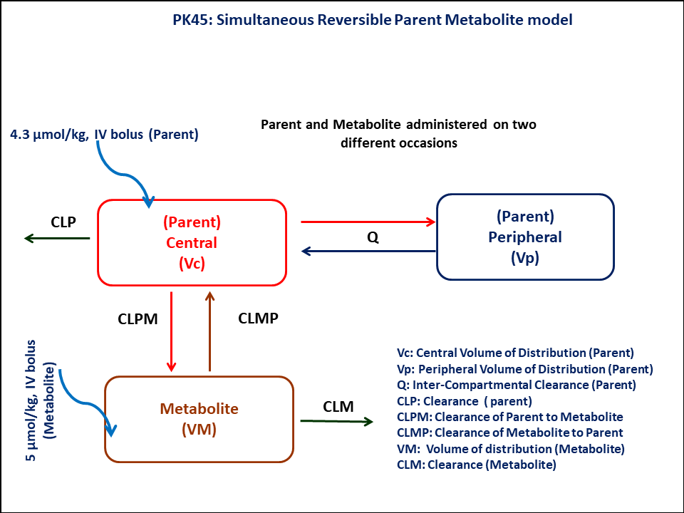
3 Libraries
Call the required libraries to get started
4 Model
This is a model describing a parent with a two-compartment disposition profile and a metabolite following a one-compartment disposition profile in the same model framework.
pk_45 = @model begin
    @metadata begin
        desc = "Two Compartment Model with Metabolite Compartment"
        timeu = u"hr"
    end

    @param begin
        """
        Volume of Distribution - Central Parent (L/kg)
        """
        tvvcp ∈ RealDomain(lower = 0)
        """
        Volume of Distribution - Peripheral Parent (L/kg)
        """
        tvvpp ∈ RealDomain(lower = 0)
        """
        Intercompartmental Clearance - Parent (L/hr/kg)
        """
        tvqp ∈ RealDomain(lower = 0)
        """
        Clearance - Parent (L/hr/kg)
        """
        tvclp ∈ RealDomain(lower = 0)
        """
        Volume of Distribution - Metabolite Parent (L/kg)
        """
        tvvcm ∈ RealDomain(lower = 0)
        """
        Clearance - Metabolite (L/hr/kg)
        """
        tvclm ∈ RealDomain(lower = 0)
        """
        Conversion of Parent to Metabolite (L/hr/kg)
        """
        tvclpm ∈ RealDomain(lower = 0)
        """
        Conversion of Metabolite to Parent (L/hr/kg)
        """
        tvclmp ∈ RealDomain(lower = 0)
        """
        Additive RUV for Parent Drug Concentration
        """
        σ_add_cp ∈ RealDomain(; lower = 0)
        """
        Additive RUV for Metabolite Drug Concentration
        """
        σ_add_met ∈ RealDomain(; lower = 0)
    end

    @pre begin
        Vcp = tvvcp
        Vpp = tvvpp
        Qp = tvqp
        Clp = tvclp
        Vcm = tvvcm
        Clm = tvclm
        Clpm = tvclpm
        Clmp = tvclmp
    end

    @dynamics begin
        Centralp' =
            (Qp / Vpp) * Peripheralp - (Qp / Vcp) * Centralp - (Clp / Vcp) * Centralp -
            (Clpm / Vcp) * Centralp + (Clmp / Vcm) * Centralm
        Peripheralp' = (Qp / Vcp) * Centralp - (Qp / Vpp) * Peripheralp
        Centralm' =
            -(Clm / Vcm) * Centralm - (Clmp / Vcm) * Centralm + (Clpm / Vcp) * Centralp
    end

    @derived begin
        cp = @. Centralp / Vcp
        met = @. Centralm / Vcm
        """
        Observed Concentration - Parent (μM)
        """
        dv_cp ~ @. Normal(cp, σ_add_cp)
        """
        Observed Concentration - Metabolite (μM)
        """
        dv_met ~ @. Normal(met, σ_add_met)
    end
end
┌ Warning: Variable `cp` is defined in the `@derived` block using `=` and hence `cp` is not used for model fitting but only returned when simulating: │ If `cp` is a random variable, it must be defined in the `@derived` block using `~`; │ if `cp` should be returned when simulating, it should be defined in the `@observed` block using `=`; │ if `cp` is an intermediate quantity that should not be returned when simulating, it should be defined using `:=`. └ @ Pumas ~/run/_work/PumasTutorials.jl/PumasTutorials.jl/custom_julia_depot/packages/Pumas/GZeMg/src/dsl/model_macro.jl:2351 ┌ Warning: Variable `met` is defined in the `@derived` block using `=` and hence `met` is not used for model fitting but only returned when simulating: │ If `met` is a random variable, it must be defined in the `@derived` block using `~`; │ if `met` should be returned when simulating, it should be defined in the `@observed` block using `=`; │ if `met` is an intermediate quantity that should not be returned when simulating, it should be defined using `:=`. └ @ Pumas ~/run/_work/PumasTutorials.jl/PumasTutorials.jl/custom_julia_depot/packages/Pumas/GZeMg/src/dsl/model_macro.jl:2351
PumasModel
  Parameters: tvvcp, tvvpp, tvqp, tvclp, tvvcm, tvclm, tvclpm, tvclmp, σ_add_cp, σ_add_met
  Random effects:
  Covariates:
  Dynamical system variables: Centralp, Peripheralp, Centralm
  Dynamical system type: Matrix exponential
  Derived: cp, met, dv_cp, dv_met
  Observed: cp, met, dv_cp, dv_met
WarningTake note of the derived block!
- Do not forget the
@. - Be sure to code for the correct Residual Unexplained Variability (RUV) in the derived block. This is an example of a model with additive RUV.
5 Parameters
Parameters provided for simulation.
tvvcp- Volume of distribution of central compartment of Parent (L/kg)tvvpp- Volume of distribution of peripheral compartment of Parent (L/kg)tvqp- Intercompartmental clearance of Parent (L/hr/kg)tvclp- Clearance of Parent (L/hr/kg)tvvcm- Volume of distribution of central compartment of Metabolite (L/kg)tvclm- Clearance of Metabolite (L/hr/kg)tvclpm- Conversion of Parent to Metabolite (L/hr/kg)tvclmp- Conversion of Metabolite to Parent (L/hr/kg)σ- Residual error
These are the initial estimates that we will be using in this model exercise. Note that tv represents the typical value for parameters.
param = (;
    tvvcp = 0.563,
    tvvpp = 0.424,
    tvqp = 0.115,
    tvclp = 0.343,
    tvvcm = 0.932,
    tvclm = 0.068,
    tvclpm = 0.015,
    tvclmp = 0.046,
    σ_add_cp = 0.002,
    σ_add_met = 0.003,
)
6 Dosage Regimen
To start the simulation process, the dosing regimen from the background section must be developed first prior to running a simulation.
The dosage regimen is specified as:
- A dose of 4.3 μmol/kg of the Parent is administered as a rapid IV Injection over 15 seconds
- A dose of 5 μmol/kg of the metabolite is administered as a rapid IV Injection over 15 seconds
This is how to establish the dosing regimen:
dr_p = DosageRegimen(4.3; cmt = 1, time = 0, duration = 0.0041)1×10 DataFrame
| Row | time | cmt | amt | evid | ii | addl | rate | duration | ss | route |
|---|---|---|---|---|---|---|---|---|---|---|
| Float64 | Int64 | Float64 | Int8 | Float64 | Int64 | Float64 | Float64 | Int8 | NCA.Route | |
| 1 | 0.0 | 1 | 4.3 | 1 | 0.0 | 0 | 1048.78 | 0.0041 | 0 | NullRoute |
This is how to create the population undergoing the dosing regimen above.
sub_p = Subject(; id = "Parent", events = dr_p)Subject
ID: Parent
Events: 1The same process will be repeated for the metabolite.
dr_m = DosageRegimen(5; cmt = 3, time = 0, duration = 0.0041)1×10 DataFrame
| Row | time | cmt | amt | evid | ii | addl | rate | duration | ss | route |
|---|---|---|---|---|---|---|---|---|---|---|
| Float64 | Int64 | Float64 | Int8 | Float64 | Int64 | Float64 | Float64 | Int8 | NCA.Route | |
| 1 | 0.0 | 3 | 5.0 | 1 | 0.0 | 0 | 1219.51 | 0.0041 | 0 | NullRoute |
sub_m = Subject(; id = "Metabolite", events = dr_m)Subject
ID: Metabolite
Events: 1This is putting both subjects together as a population.
sub = [sub_p, sub_m]Population
Subjects: 2
Observations: 7 Simulation
We are going to simulate the parent and metabolite concentration profiles.
Note
Random.seed!()
The Random.seed! function is included here for purposes of reproducibility of the simulation in this tutorial. Specification of a seed value would not be required in a Pumas workflow that is estimating model parameters.
Random.seed!(123)sim_sub = simobs(pk_45, sub, param, obstimes = 0.1:0.001:31)Simulated population (Vector{<:Subject})
Simulated subjects: 2
Simulated variables: cp, met, dv_cp, dv_met8 Visualization
From the plots below, we can observe the parent and metabolite concentration profiles in the system.
@chain DataFrame(sim_sub) begin
    dropmissing(:cp)
    data(_) *
    mapping(
        :time => "Time (hours)",
        :cp => "Parent Concentration (μM)",
        color = :id => "",
    ) *
    visual(Lines; linewidth = 4)
    draw(;
        figure = (; fontsize = 22),
        axis = (;
            yscale = log10,
            ytickformat = i -> (@. string(round(i; digits = 1))),
            xticks = 0:5:35,
        ),
        legend = (; position = :bottom),
    )
end
@chain DataFrame(sim_sub) begin
    dropmissing(:met)
    data(_) *
    mapping(
        :time => "Time (hours)",
        :met => "Metabolite Concentration (μM)",
        color = :id => "",
    ) *
    visual(Lines; linewidth = 4)
    draw(;
        figure = (; fontsize = 22),
        axis = (;
            yscale = log10,
            ytickformat = i -> (@. string(round(i; digits = 1))),
            xticks = 0:5:35,
        ),
        legend = (; position = :bottom),
    )
end
9 Population Simulation
This block updates the parameters of the model to increase intersubject variability in parameters and defines timepoints for the prediction of concentrations. The results are written to a CSV file.
These are the initial parameters that will be used and the creation of the populations for the parent and the metabolite.
par = (
    tvvcp = 0.563,
    tvvpp = 0.424,
    tvqp = 0.115,
    tvclp = 0.343,
    tvvcm = 0.932,
    tvclm = 0.068,
    tvclpm = 0.015,
    tvclmp = 0.046,
    σ_add_cp = 0.002,
    σ_add_met = 0.003,
)

dr_p = DosageRegimen(4.3; cmt = 1, time = 0, duration = 0.0041)
pop_p = map(
    i -> Subject(
        id = i,
        events = dr_p,
        time = [0.0042, 0.0333, 0.1667, 0.5, 1, 2, 2.75, 5, 7, 24, 31],
    ),
    1:24,
)
dr_m = DosageRegimen(5; cmt = 3, time = 0, duration = 0.0041)
pop_m = map(
    i -> Subject(
        id = i,
        events = dr_m,
        time = [0.0042, 0.0333, 0.1333, 0.25, 0.75, 2, 4, 7, 12, 23],
    ),
    25:48,
)
This is the evaluation for the overall population.
pop = [pop_p; pop_m]

Random.seed!(1234)
sim_pop = simobs(pk_45, pop, par)
sim_plot(sim_pop)

df_sim = DataFrame(sim_pop)

#CSV.write("pk_45.csv", df_sim)
NoteSaving the Simulation Results
With the CSV.write function, you can input the name of the dataframe (df_sim) and the file name of your choice (pk_45.csv) to save the file to your local directory or repository.
10 Conclusion
Constructing a multi-part model showcasing a parent/metabolite relationship with two different disposition profiles involves:
- understanding the process of how the metabolite is passed through the system,
- translating processes for both parent and metabolite into ODEs using Pumas, and
- simulating the model in a single patient for evaluation.