PK46 - Long Infusion and Short Half-Life

1 Background

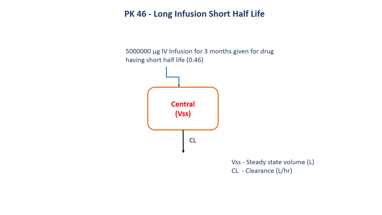
Structural model - Long infusion short half life one compartment model
Route of administration - IV infusion
Dosage Regimen - 500000 μg
Number of Subjects - 1

2 Learning Outcome

This exercise deals with the drug having a short half life.

3 Objectives

To build a model for a drug having a short half life given as a very long infusion of up to 3 months.

4 Libraries

Call the necessary libraries to get started.

using Random
using Pumas
using PumasUtilities
using AlgebraOfGraphics
using CairoMakie
using CSV
using DataFramesMeta
using Dates

5 Model

To build a one compartment model for a drug having a short half life given a long infusion for 3 months.

pk_46 = @model begin
    @metadata begin
        desc = "One Compartment Model"
        timeu = u"hr"
    end

    @param begin
        """
        Volume at Steady State (L)
        """
        tvvss ∈ RealDomain(lower = 0)
        """
        Clearance (L/hr)
        """
        tvcl ∈ RealDomain(lower = 0)
        Ω ∈ PDiagDomain(2)
        """
        Additive Error
        """
        σ_add ∈ RealDomain(lower = 0)
    end

    @random begin
        η ~ MvNormal(Ω)
    end

    @pre begin
        Vss = tvvss * exp(η[1])
        Cl = tvcl * exp(η[2])
    end

    @dynamics begin
        Central' = -(Cl / Vss) * Central
    end


    @derived begin
        cp = @. Central / Vss
        """
        Observed Concentration (μg/L)
        """
        dv ~ @. Normal(cp, σ_add)
    end
end

PumasModel
  Parameters: tvvss, tvcl, Ω, σ_add
  Random effects: η
  Covariates: 
  Dynamical system variables: Central
  Dynamical system type: Matrix exponential
  Derived: cp, dv
  Observed: cp, dv

6 Parameters

Parameters provided for simulation are as below. Note that tv represents the typical value for parameters.

Vss - Steady state volume (L)
CL - Clearance (L/hr)

param = (; tvvss = 35.6, tvcl = 61, Ω = Diagonal([0.04, 0.04]), σ_add = 0.196337)

7 Dosage Regimen

A dose of 500000 μg was given as an Intravenous Infusion to a single subject for over 3 months.

ev1 = DosageRegimen(500000, time = 0, cmt = 1, duration = 2016)

1×10 DataFrame

Row	time	cmt	amt	evid	ii	addl	rate	duration	ss	route
	Float64	Int64	Float64	Int8	Float64	Int64	Float64	Float64	Int8	NCA.Route
1	0.0	1	500000.0	1	0.0	0	248.016	2016.0	0	NullRoute

sub1 = Subject(id = 1, events = ev1)

Subject
  ID: 1
  Events: 2

8 Simulation

Simulate the data after the administration of an infusion

Random.seed!(123)

The random effects are zero’ed out since we are simulating a single subject

zfx = zero_randeffs(pk_46, sub1, param)

(η = [0.0, 0.0],)

sim_sub1 = simobs(pk_46, sub1, param, zfx, obstimes = 0.5:0.1:2100)

SimulatedObservations
  Simulated variables: cp, dv
  Time: 0.5:0.1:2100.0

9 Visualization

@chain DataFrame(sim_sub1) begin
    dropmissing(:cp)
    data(_) *
    mapping(:time => "Time (hours)", :cp => "Concentration (μg/L)") *
    visual(Lines; linewidth = 4)
    draw(; figure = (; fontsize = 22), axis = (; xticks = 0:500:2000))
end

The plot below shows the decline in the concentrations after the end of the infusion

@chain DataFrame(sim_sub1) begin
    @rsubset 2016 ≤ :time < 2020
    data(_) *
    mapping(:time => "Time (hours)", :cp => "Concentration (μg/L)") *
    visual(ScatterLines; linewidth = 4)
    draw(;
        axis = (;
            yscale = Makie.Symlog10(10.0),
            limits = (nothing, (-0.1, nothing)),
            xticks = 2015:1:2020,
        ),
    )
end

10 Simulating a Population

par = (; tvvss = 35.6, tvcl = 61, Ω = Diagonal([0.0125, 0.0224]), σ_add = 0.196337)

ev1 = DosageRegimen(500000, time = 0, cmt = 1, duration = 2016)
pop = map(i -> Subject(id = i, events = ev1), 1:72)

Random.seed!(1234)
sim_pop =
    simobs(pk_46, pop, par, obstimes = [0.5, 24, 96, 168, 672, 2016, 2016.5, 2017, 2018])

df_sim = DataFrame(sim_pop)
#CSV.write("pk_46.csv", df_sim)