using Random
using Pumas
using PumasUtilities
using CairoMakie
using AlgebraOfGraphics
using DataFramesMeta
using CSV
using Dates
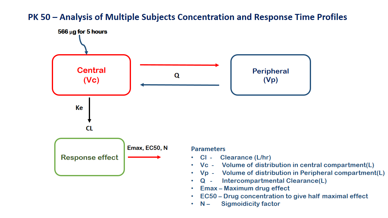
PK50 - Analysis of multiple subjects concentration and response-time profiles
1 Background
- Structural model - Two compartment Model
- Route of administration - IV Infusion
- Dosage Regimen - 566 μg
- Number of Subjects - 12
2 Learning Outcome
To analyze and interpret exposure and effect with plasma protein binding as a co-covariate of PK parameters and exposure
3 Objectives
To build a sequential PKPD model for a drug considering fraction unbound as a covariate
4 Libraries
Call the necessary libraries to get started.
5 Model
A sequential two compartment PKPD model for a drug after infusion over 5 hours
pk_50 = @model begin
    @metadata begin
        desc = "Two Compartment Model"
        timeu = u"hr"
    end

    @param begin
        """
        Clearance (L/hr)
        """
        tvcl ∈ RealDomain(lower = 0)
        """
        Intercompartmental Clearance (L/hr)
        """
        tvcld ∈ RealDomain(lower = 0)
        """
        Volume of Disttibution - Central (L)
        """
        tvvc ∈ RealDomain(lower = 0)
        """
        Volume of Disttibution - Peripheral (L)
        """
        tvvt ∈ RealDomain(lower = 0)
        """
        Concentration which produces 50% effect (μg/L)
        """
        tvec50 ∈ RealDomain(lower = 0)
        """
        Maximum Effect
        """
        tvemax ∈ RealDomain(lower = 0)
        """
        Sigmoidicity factor
        """
        tvsigma ∈ RealDomain(lower = 0)
        Ω ∈ PDiagDomain(7)
        """
        Proportional RUV
        """
        σ_prop ∈ RealDomain(lower = 0)
        """
        Additive RUV
        """
        σ_add ∈ RealDomain(lower = 0)
    end

    @random begin
        η ~ MvNormal(Ω)
    end

    @covariates fu

    @pre begin
        Cl = tvcl * (1 / fu) * exp(η[1])
        Cld = tvcld * (1 / fu) * exp(η[2])
        Vc = tvvc * (1 / fu) * exp(η[3])
        Vt = tvvt * (1 / fu) * exp(η[4])
        EC50 = tvec50 * (fu) * exp(η[5])
        Emax = tvemax * exp(η[6])
        sigma = tvsigma * exp(η[7])
    end

    @dynamics begin
        Central' = -(Cl / Vc) * Central - (Cld / Vc) * Central + (Cld / Vt) * Peripheral
        Peripheral' = (Cld / Vc) * Central - (Cld / Vt) * Peripheral
    end

    @derived begin
        cp = @. Central / Vc
        """
        Observed Concentration (μg/L)
        """
        dv_cp ~ ProportionalNormal.(cp, sqrt(σ_prop))
        ef = @. Emax * (cp^sigma) / (EC50^sigma + cp^sigma)
        """
        Observed Response
        """
        dv_ef ~ @. Normal(ef, σ_add)
    end
end
┌ Warning: Variable `cp` is defined in the `@derived` block using `=` and hence `cp` is not used for model fitting but only returned when simulating: │ If `cp` is a random variable, it must be defined in the `@derived` block using `~`; │ if `cp` should be returned when simulating, it should be defined in the `@observed` block using `=`; │ if `cp` is an intermediate quantity that should not be returned when simulating, it should be defined using `:=`. └ @ Pumas ~/run/_work/PumasTutorials.jl/PumasTutorials.jl/custom_julia_depot/packages/Pumas/GZeMg/src/dsl/model_macro.jl:2351 ┌ Warning: Variable `ef` is defined in the `@derived` block using `=` and hence `ef` is not used for model fitting but only returned when simulating: │ If `ef` is a random variable, it must be defined in the `@derived` block using `~`; │ if `ef` should be returned when simulating, it should be defined in the `@observed` block using `=`; │ if `ef` is an intermediate quantity that should not be returned when simulating, it should be defined using `:=`. └ @ Pumas ~/run/_work/PumasTutorials.jl/PumasTutorials.jl/custom_julia_depot/packages/Pumas/GZeMg/src/dsl/model_macro.jl:2351
PumasModel
  Parameters: tvcl, tvcld, tvvc, tvvt, tvec50, tvemax, tvsigma, Ω, σ_prop, σ_add
  Random effects: η
  Covariates: fu
  Dynamical system variables: Central, Peripheral
  Dynamical system type: Matrix exponential
  Derived: cp, dv_cp, ef, dv_ef
  Observed: cp, dv_cp, ef, dv_ef
6 Parameters
Parameters provided for simulation are as below. Note that tv represents the typical value for parameters.
Cl- Clearance (L/hr)Vc- Volume of distribution in central compartment (L)Vp- Volume of distribution in Peripheral compartment (L)Q- Intercompartmental Clearance (L/hr)EC50- Concentration which produces 50% effect (μg/L)Emax- Maximum Effectsigma- Sigmoidicity factor
param = (;
    tvcl = 11.4,
    tvcld = 4.35,
    tvvc = 19.9,
    tvvt = 30.9,
    tvec50 = 1.8,
    tvemax = 2.1,
    tvsigma = 2.1,
    Ω = Diagonal([0.0784, 0.1521, 0.0841, 0.1225, 0.16, 0.36, 0.09]),
    σ_prop = 0.00,
    σ_add = 0.00,
)
7 Dosage Regimen
A group of 12 subjects is administered a dose of 566 μg infused over 5 hours
## Total Plasma Concentration
ev1 = DosageRegimen(566, cmt = 1, time = 0, duration = 5)
1×10 DataFrame
| Row | time | cmt | amt | evid | ii | addl | rate | duration | ss | route |
|---|---|---|---|---|---|---|---|---|---|---|
| Float64 | Int64 | Float64 | Int8 | Float64 | Int64 | Float64 | Float64 | Int8 | NCA.Route | |
| 1 | 0.0 | 1 | 566.0 | 1 | 0.0 | 0 | 113.2 | 5.0 | 0 | NullRoute |
sub_total =
    map(i -> Subject(id = i, events = ev1, covariates = (fu = 1, group = "Total")), 1:12)
Population
Subjects: 12
Covariates: fu, group
Observations: ## Unbound Plasma Concentration
fu1 = Normal(0.016, 0.0049)Random.seed!(1234)fu = rand(fu1, 12)12-element Vector{Float64}:
0.02075621601139055
0.011201829783477522
0.02041911832961106
0.015839264666701266
0.01305611810555775
0.008918632135097459
0.029266377314407323
0.023469794530834417
0.014992411157462667
0.01977644555794693
0.010051693161265264
0.02134834305213556df_unbound = map(
((i, fui),) -> DataFrame(
id = i,
amt = 566,
time = 0,
cmt = 1,
evid = 1,
rate = 113.2,
dv_cp = missing,
dv_ef = missing,
fu = fui,
group = "Unbound",
),
zip(1:12, fu),
)df1_unbound = vcat(DataFrame.(df_unbound)...)12×10 DataFrame
| Row | id | amt | time | cmt | evid | rate | dv_cp | dv_ef | fu | group |
|---|---|---|---|---|---|---|---|---|---|---|
| Int64 | Int64 | Int64 | Int64 | Int64 | Float64 | Missing | Missing | Float64 | String | |
| 1 | 1 | 566 | 0 | 1 | 1 | 113.2 | missing | missing | 0.0207562 | Unbound |
| 2 | 2 | 566 | 0 | 1 | 1 | 113.2 | missing | missing | 0.0112018 | Unbound |
| 3 | 3 | 566 | 0 | 1 | 1 | 113.2 | missing | missing | 0.0204191 | Unbound |
| 4 | 4 | 566 | 0 | 1 | 1 | 113.2 | missing | missing | 0.0158393 | Unbound |
| 5 | 5 | 566 | 0 | 1 | 1 | 113.2 | missing | missing | 0.0130561 | Unbound |
| 6 | 6 | 566 | 0 | 1 | 1 | 113.2 | missing | missing | 0.00891863 | Unbound |
| 7 | 7 | 566 | 0 | 1 | 1 | 113.2 | missing | missing | 0.0292664 | Unbound |
| 8 | 8 | 566 | 0 | 1 | 1 | 113.2 | missing | missing | 0.0234698 | Unbound |
| 9 | 9 | 566 | 0 | 1 | 1 | 113.2 | missing | missing | 0.0149924 | Unbound |
| 10 | 10 | 566 | 0 | 1 | 1 | 113.2 | missing | missing | 0.0197764 | Unbound |
| 11 | 11 | 566 | 0 | 1 | 1 | 113.2 | missing | missing | 0.0100517 | Unbound |
| 12 | 12 | 566 | 0 | 1 | 1 | 113.2 | missing | missing | 0.0213483 | Unbound |
pop12_unbound =
    read_pumas(df1_unbound, observations = [:dv_cp, :dv_ef], covariates = [:fu, :group])
Population
Subjects: 12
Covariates: fu, group
Observations: dv_cp, dv_efpop24_sub = [sub_total; pop12_unbound]8 Simulation
Simulate the data and create a DataFrame with specific data points.
sim_pop24_sub = simobs(
    pk_50,
    pop24_sub,
    param,
    obstimes = [
        0.1,
        0.25,
        0.5,
        0.75,
        1,
        2,
        3,
        4,
        4.999,
        5.03,
        5.08,
        5.17,
        5.25,
        5.5,
        5.75,
        6,
        6.5,
        7,
        8,
        9,
        10,
        12,
        24,
    ],
)
Simulated population (Vector{<:Subject})
Simulated subjects: 24
Simulated variables: cp, dv_cp, ef, dv_efdf50 = DataFrame(sim_pop24_sub)
first(df50, 5)5×34 DataFrame
| Row | id | time | cp | dv_cp | ef | dv_ef | evid | amt | cmt | rate | duration | ss | ii | route | fu | group | tad | dosenum | Central | Peripheral | η₁ | η₂ | η₃ | η₄ | η₅ | η₆ | η₇ | Cl | Cld | Vc | Vt | EC50 | Emax | sigma |
|---|---|---|---|---|---|---|---|---|---|---|---|---|---|---|---|---|---|---|---|---|---|---|---|---|---|---|---|---|---|---|---|---|---|---|
| String | Float64 | Float64? | Float64? | Float64? | Float64? | Int64? | Float64? | Symbol? | Float64? | Float64? | Int8? | Float64? | NCA.Route? | Float64? | String? | Float64? | Int64? | Float64? | Float64? | Float64? | Float64? | Float64? | Float64? | Float64? | Float64? | Float64? | Float64? | Float64? | Float64? | Float64? | Float64? | Float64? | Float64? | |
| 1 | 1 | 0.0 | missing | missing | missing | missing | 1 | 566.0 | Central | 113.2 | 5.0 | 0 | 0.0 | NullRoute | 1.0 | Total | 0.0 | 1 | missing | missing | 0.00047241 | 0.0665458 | -0.316058 | 0.103237 | -0.0357759 | 0.80884 | 0.00104036 | 11.4054 | 4.64932 | 14.5074 | 34.2605 | 1.73674 | 4.71513 | 2.10219 |
| 2 | 1 | 0.1 | 0.738717 | 0.738717 | 0.670537 | 0.670537 | 0 | 0.0 | missing | 0.0 | 0.0 | 0 | 0.0 | missing | 1.0 | Total | 0.1 | 1 | 10.7169 | 0.174091 | 0.00047241 | 0.0665458 | -0.316058 | 0.103237 | -0.0357759 | 0.80884 | 0.00104036 | 11.4054 | 4.64932 | 14.5074 | 34.2605 | 1.73674 | 4.71513 | 2.10219 |
| 3 | 1 | 0.25 | 1.7049 | 1.7049 | 2.31171 | 2.31171 | 0 | 0.0 | missing | 0.0 | 0.0 | 0 | 0.0 | missing | 1.0 | Total | 0.25 | 1 | 24.7337 | 1.02434 | 0.00047241 | 0.0665458 | -0.316058 | 0.103237 | -0.0357759 | 0.80884 | 0.00104036 | 11.4054 | 4.64932 | 14.5074 | 34.2605 | 1.73674 | 4.71513 | 2.10219 |
| 4 | 1 | 0.5 | 3.0017 | 3.0017 | 3.58141 | 3.58141 | 0 | 0.0 | missing | 0.0 | 0.0 | 0 | 0.0 | missing | 1.0 | Total | 0.5 | 1 | 43.547 | 3.71731 | 0.00047241 | 0.0665458 | -0.316058 | 0.103237 | -0.0357759 | 0.80884 | 0.00104036 | 11.4054 | 4.64932 | 14.5074 | 34.2605 | 1.73674 | 4.71513 | 2.10219 |
| 5 | 1 | 0.75 | 3.99194 | 3.99194 | 4.01682 | 4.01682 | 0 | 0.0 | missing | 0.0 | 0.0 | 0 | 0.0 | missing | 1.0 | Total | 0.75 | 1 | 57.9128 | 7.61798 | 0.00047241 | 0.0665458 | -0.316058 | 0.103237 | -0.0357759 | 0.80884 | 0.00104036 | 11.4054 | 4.64932 | 14.5074 | 34.2605 | 1.73674 | 4.71513 | 2.10219 |
9 Visualization
Plot a graph of Concentrations vs Time
@chain df50 begin
    dropmissing!(:cp)
    data(_) *
    mapping(
        :time => "Time (hrs)",
        :cp => "Concentration (μg/L)",
        color = :group => "",
        group = :id,
    ) *
    visual(Lines, linewidth = 2)
    draw(;
        axis = (;
            xticks = 0:5:25,
            yscale = log10,
            ytickformat = i -> (@. string(round(i; sigdigits = 1))),
        ),
        figure = (; fontsize = 22),
    )
end
Plot a graph of Response vs Concentrations
@chain df50 begin
    dropmissing!(:cp)
    data(_) *
    mapping(
        :cp => "Concentration (μg/L)",
        :ef => "Response",
        color = :group => "",
        group = :id,
    ) *
    visual(Lines, linewidth = 2)
    draw(;
        axis = (; xscale = log10, xtickformat = i -> (@. string(round(i; sigdigits = 1)))),
        figure = (; fontsize = 22),
    )
end
Question - 1 and 2
- What infusion rate do you aim at in the present patient population during the first hour to reach a plasma concentration > 10 μg/L and < 50 μg/L.
Ans: We have targeted a plasma concentration of 30 μg/L and thus the dose required to achieve that concentration is 784 μg given as an IV-infusion over 1 hour, followed by a 7843 μg given as an IV-infusion over 23 hours
- What Infusion rate is needed to remain at the steady state plasma concentration between 1 and 24 hours?
Ans: An infusion rate of 341 μg/hr is given to achieve the steady-state plasma concentration of 30 μg/L
## Dosage Regimen - Total Plasma Concentration
ev12 = DosageRegimen([784, 7843], cmt = 1, time = [0, 1], rate = [784, 341])
pop12 = Population(
    map(i -> Subject(id = i, events = ev12, covariates = (fu = 1, group = "Total")), 1:12),
)

## Simulation
Random.seed!(123)
sim12 = simobs(
    pk_50,
    pop12,
    param,
    obstimes = [
        0.1,
        0.25,
        0.5,
        0.75,
        1,
        2,
        3,
        4,
        4.999,
        5.03,
        5.08,
        5.17,
        5.25,
        5.5,
        5.75,
        6,
        6.5,
        7,
        8,
        9,
        10,
        12,
        24,
    ],
)
df12 = DataFrame(sim12)
dropmissing!(df12, :cp)

@chain df12 begin
    data(_) *
    mapping(:time => "Time (hrs)", :cp => "Concentration (μg/L)", group = :id) *
    visual(Lines, linewidth = 2)
    draw(;
        axis = (;
            xticks = 0:5:25,
            yscale = log10,
            ytickformat = i -> (@. string(round(i; sigdigits = 1))),
        ),
        figure = (; fontsize = 22),
    )
end
Question - 3
- What unbound plasma concentration are reached (given the range) with the infusion rates calculated for the 1+23 hrs regimen? How does the variability seen in the predicted exposure at 1 and 24 hours compare between total and unbound concentration?
## Dosage Regimen - Unbound Plasma Concentration
df_3 = map(
    ((i, fui),) -> DataFrame(
        id = i,
        amt = [784, 7800],
        time = [0, 1],
        cmt = [1, 1],
        evid = [1, 1],
        rate = [784, 339],
        dv_cp = missing,
        dv_ef = missing,
        fu = fui,
        group = "Unbound",
    ),
    zip(1:12, fu),
)
df1_3 = vcat(DataFrame.(df_3)...)
pop_3_unbound =
    read_pumas(df1_3, observations = [:dv_cp, :dv_ef], covariates = [:fu, :group])

pop_3 = [pop12; pop_3_unbound]

## Simulation
Random.seed!(12345)
sim3 = simobs(
    pk_50,
    pop_3,
    param,
    obstimes = [
        0.1,
        0.25,
        0.5,
        0.75,
        1.0,
        2,
        3,
        4,
        4.999,
        5.03,
        5.08,
        5.17,
        5.25,
        5.5,
        5.75,
        6,
        6.5,
        7,
        8,
        9,
        10,
        12,
        24,
    ],
)
df_sim3 = DataFrame(sim3)

@chain df_sim3 begin
    dropmissing!(:cp)
    data(_) *
    mapping(
        :time => "Time (hrs)",
        :cp => "Concentration (μg/L)",
        color = :group => "",
        group = :id,
    ) *
    visual(Lines, linewidth = 2)
    draw(;
        axis = (;
            xticks = 0:5:25,
            yscale = log10,
            ytickformat = i -> (@. string(round(i; sigdigits = 1))),
        ),
        figure = (; fontsize = 22),
    )
end
Question - 4
- What exposure is needed in the new 1 + 23 hours infusion study to establish a response greater than one(1) Response unit?
Ans: The new 1 + 23 hr infusion chosen to achieve a steady-state concentration of 30 μg/L will help to achieve a response greater than 1 unit.
@chain df_sim3 begin
    dropmissing!(:cp)
    data(_) *
    mapping(
        :cp => "Concentration (μg/L)",
        :ef => "Response",
        color = :group => "",
        group = :id,
    ) *
    visual(Lines, linewidth = 2)
    draw(;
        axis = (; xscale = log10, xtickformat = i -> (@. string(round(i; sigdigits = 1)))),
        figure = (; fontsize = 22),
    )
end