using Pumas
using PumasUtilities
using Random
using CairoMakie
using AlgebraOfGraphics
using DataFramesMeta
using CSV
PK51 - Multi-Compartment Drug/Metabolite
1 Learning Outcome
In this tutorial, you will gain a greater appreciation and learn about two compartment parent - metabolite kinetics.
With this modeling exercise, a drug is administered both IV and orally at different occasions to different subjects, and plasma data is collected. The concentrations are obtained for both the drugs and metabolites.
2 Objectives
In this tutorial, you will learn how to build a multi compartment drug/metabolite model and to simulate the model for different subjects and dosage regimens.
3 Background
Before constructing a model, it is important to establish the process the model will follow and a scenario for the simulation.
Below is the scenario for this tutorial:
- Structural model - Multi-Compartment drug/metabolite
- Route of administration - IV administration to one subject and oral administration to another subject
- Dosage Regimen - 5000 mg IV and 8000 mg Oral
- Number of Subjects - 2
This diagram describes how such an administered dose will be handled, which facilitates building the model. 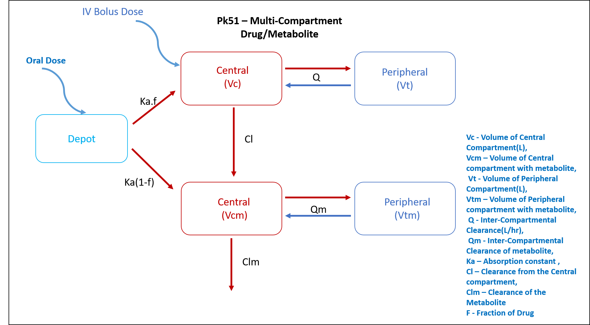
4 Libraries
Call the required libraries to get started.
5 Model
In this two compartment model, we administer the dose to the oral and central compartments on two different occasions.
pk_51 = @model begin
    @metadata begin
        desc = "Two Compartment Model with Metabolite Compartment"
        timeu = u"hr"
    end

    @param begin
        """
        Volume of Central Compartment (L)
        """
        tvvc ∈ RealDomain(lower = 0)
        """
        Clearance (L/hr)
        """
        tvcl ∈ RealDomain(lower = 0)
        """
        Inter Compartmental Clearance (L/hr)
        """
        tvcld ∈ RealDomain(lower = 0)
        """
        Volume of Peripheral Compartment (L)
        """
        tvvt ∈ RealDomain(lower = 0)
        """
        Volume of Central Compartment of Metabolite (L)
        """
        tvvcm ∈ RealDomain(lower = 0)
        """
        Clearance of metabolite (L/hr)
        """
        tvclm ∈ RealDomain(lower = 0)
        """
        Inter Compartmental Clearance of Metabolite (L/hr)
        """
        tvcldm ∈ RealDomain(lower = 0)
        """
        Volume of Peripheral Compartment of Metabolite (L)
        """
        tvvtm ∈ RealDomain(lower = 0)
        """
        Absorption rate constant (hr⁻¹)
        """
        tvka ∈ RealDomain(lower = 0)
        """
        Fraction of drug absorbed
        """
        tvf ∈ RealDomain(lower = 0)
        """
        Lag time (hr)
        """
        tvlag ∈ RealDomain(lower = 0)
        Ω ∈ PDiagDomain(7)
        """
        Proportional RUV - Plasma
        """
        σ²_prop_cp ∈ RealDomain(lower = 0)
        """
        Proportional RUV - Metabolite
        """
        σ²_prop_met ∈ RealDomain(lower = 0)
    end

    @random begin
        η ~ MvNormal(Ω)
    end

    @pre begin
        Vc = tvvc * exp(η[1])
        Cl = tvcl * exp(η[2])
        Cld = tvcld * exp(η[3])
        Vt = tvvt * exp(η[4])
        Vcm = tvvcm
        Clm = tvclm * exp(η[5])
        Cldm = tvcldm
        Vtm = tvvtm * exp(η[6])
        Ka = tvka * exp(η[7])
    end

    @dosecontrol begin
        bioav = (Depot = tvf, Metabolite = (1 - tvf))
        lags = (Depot = tvlag,)
    end

    @dynamics begin
        Depot' = -Ka * Depot
        Central' =
            Ka * Depot - (Cl / Vc) * Central - (Cld / Vc) * Central +
            (Cld / Vt) * Peripheral
        Peripheral' = (Cld / Vc) * Central - (Cld / Vt) * Peripheral
        Metabolite' =
            Ka * Depot + (Cl / Vc) * Central - (Clm / Vcm) * Metabolite -
            (Cldm / Vcm) * Metabolite + (Cldm / Vtm) * PeriMetabolite
        PeriMetabolite' = (Cldm / Vcm) * Metabolite - (Cldm / Vtm) * PeriMetabolite
    end

    @derived begin
        cp = @. Central / Vc
        met = @. Metabolite / Vcm
        """
        Observed Concentration (...)
        """
        dv_cp ~ ProportionalNormal.(cp, sqrt(σ²_prop_cp))
        """
        Observed Concentration (...)
        """
        dv_met ~ ProportionalNormal.(met, sqrt(σ²_prop_met))
    end
end
┌ Warning: Variable `cp` is defined in the `@derived` block using `=` and hence `cp` is not used for model fitting but only returned when simulating: │ If `cp` is a random variable, it must be defined in the `@derived` block using `~`; │ if `cp` should be returned when simulating, it should be defined in the `@observed` block using `=`; │ if `cp` is an intermediate quantity that should not be returned when simulating, it should be defined using `:=`. └ @ Pumas ~/run/_work/PumasTutorials.jl/PumasTutorials.jl/custom_julia_depot/packages/Pumas/GZeMg/src/dsl/model_macro.jl:2351 ┌ Warning: Variable `met` is defined in the `@derived` block using `=` and hence `met` is not used for model fitting but only returned when simulating: │ If `met` is a random variable, it must be defined in the `@derived` block using `~`; │ if `met` should be returned when simulating, it should be defined in the `@observed` block using `=`; │ if `met` is an intermediate quantity that should not be returned when simulating, it should be defined using `:=`. └ @ Pumas ~/run/_work/PumasTutorials.jl/PumasTutorials.jl/custom_julia_depot/packages/Pumas/GZeMg/src/dsl/model_macro.jl:2351
PumasModel
  Parameters: tvvc, tvcl, tvcld, tvvt, tvvcm, tvclm, tvcldm, tvvtm, tvka, tvf, tvlag, Ω, σ²_prop_cp, σ²_prop_met
  Random effects: η
  Covariates:
  Dynamical system variables: Depot, Central, Peripheral, Metabolite, PeriMetabolite
  Dynamical system type: Matrix exponential
  Derived: cp, met, dv_cp, dv_met
  Observed: cp, met, dv_cp, dv_met
6 Parameters
The parameters are as given below.
Cl- Clearance (L/hr)Clm- Clearance of metabolite (L/hr)Cld- Inter Compartmental Clearance (L/hr)Cldm- Inter Compartmental Clearance of metabolite (L/hr)Vc- Volume of Central Compartment (L)Vcm- Volume of Central Compartment of Metabolite (L)f- Fraction of drug absorbedlags- Lag time (hr)Ka- Absorption rate constant (hr⁻¹)Vt- Volume of Peripheral Compartment (L)Vtm- Volume of Peripheral Compartment of metabolite (L)Ω- Between Subject Variabilityσ- Residual error
These are the initial estimates we will be using in this model exercise. Note that tv represents the typical value for parameters.
param = (;
    tvvc = 18.7,
    tvcl = 0.55,
    tvcld = 0.073,
    tvvt = 10,
    tvvcm = 4.9,
    tvclm = 0.08,
    tvcldm = 0.58,
    tvvtm = 55,
    tvka = 0.03,
    tvf = 0.24,
    tvlag = 21,
    Ω = Diagonal([0.01, 0.01, 0.01, 0.01, 0.01, 0.01, 0.01]),
    σ²_prop_cp = 0.015,
    σ²_prop_met = 0.015,
)
7 Dosage Regimen
To start the simulation process, the dosing regimen from the background section must be developed first prior to running a simulation.
7.1 IV
A single dose of 5000 mg given as a rapid IV injection.
The dosage regimen is specified as:
ev1 = DosageRegimen(5000; time = 0, cmt = 2)1×10 DataFrame
| Row | time | cmt | amt | evid | ii | addl | rate | duration | ss | route |
|---|---|---|---|---|---|---|---|---|---|---|
| Float64 | Int64 | Float64 | Int8 | Float64 | Int64 | Float64 | Float64 | Int8 | NCA.Route | |
| 1 | 0.0 | 2 | 5000.0 | 1 | 0.0 | 0 | 0.0 | 0.0 | 0 | NullRoute |
This is how to create the single subject undergoing the dosing regimen above.
sub1 = Subject(; id = 1, events = ev1)Subject
ID: 1
Events: 17.2 Oral
A single dose of 8000 mg given orally.
The dosage regimen is specified as:
ev2 = DosageRegimen(8000; time = 0, cmt = 1)1×10 DataFrame
| Row | time | cmt | amt | evid | ii | addl | rate | duration | ss | route |
|---|---|---|---|---|---|---|---|---|---|---|
| Float64 | Int64 | Float64 | Int8 | Float64 | Int64 | Float64 | Float64 | Int8 | NCA.Route | |
| 1 | 0.0 | 1 | 8000.0 | 1 | 0.0 | 0 | 0.0 | 0.0 | 0 | NullRoute |
This is how to create the single subject undergoing the dosing regimen above.
sub2 = Subject(; id = 2, events = ev2)Subject
ID: 2
Events: 1This is how to put both subjects together into a population.
pop2_sub = [sub1, sub2]Population
Subjects: 2
Observations: 8 Simulation
Simulate using the simobs function.
Note
Random.seed!()
The Random.seed! function is included here for purposes of reproducibility of the simulation in this tutorial. Specification of a seed value would not be required in a Pumas workflow that is estimating model parameters.
Random.seed!(123)sim_pop2_sub = simobs(pk_51, pop2_sub, param, obstimes = 0.1:0.1:1500)Simulated population (Vector{<:Subject})
Simulated subjects: 2
Simulated variables: cp, met, dv_cp, dv_met9 Visualization
In the following plots below, we can see the concentration profiles of the parent drug and the metabolite.
@chain DataFrame(sim_pop2_sub) begin
    dropmissing(:cp)
    data(_) *
    mapping(
        :time => "Time (hours)",
        :cp => "Parent Concentration (-)";
        color = :id => nonnumeric => "ID",
    ) *
    visual(Lines; linewidth = 4)
    draw(; figure = (; fontsize = 22), axis = (; xticks = 0:150:1500))
end
@chain DataFrame(sim_pop2_sub) begin
    dropmissing(:met)
    data(_) *
    mapping(
        :time => "Time (hours)",
        :met => "Metabolite Concentration (-)";
        color = :id => nonnumeric => "ID",
    ) *
    visual(Lines; linewidth = 4)
    draw(; figure = (; fontsize = 22), axis = (; xticks = 0:150:1500))
end
10 Population Simulation
This block updates the parameters of the model to increase intersubject variability in parameters and defines timepoints for prediction of concentrations. The results are written to a CSV file.
Creating a larger population for the simulation and utilizing the following initial estimates for the simulation below:
par = (
    tvvc = 18.7,
    tvcl = 0.55,
    tvcld = 0.073,
    tvvt = 10,
    tvvcm = 4.9,
    tvclm = 0.08,
    tvcldm = 0.58,
    tvvtm = 55,
    tvka = 0.03,
    tvf = 0.24,
    tvlag = 21,
    Ω = Diagonal([0.04, 0.02, 0.02, 0.03, 0.02, 0.04, 0.04]),
    σ²_prop_cp = 0.04,
    σ²_prop_met = 0.09,
)

ev1 = DosageRegimen(5000, time = 0, cmt = 2)
pop1 = map(i -> Subject(id = i, events = ev1), 1:25)

ev2 = DosageRegimen(8000, time = 0, cmt = 1)
pop2 = map(i -> Subject(id = 1, events = ev2), 26:50)
Simulating the population and obtaining the results.
pop = [pop1; pop2]

Random.seed!(1234)
sim_pop = simobs(
    pk_51,
    pop,
    par,
    obstimes = [2, 5, 10, 15, 30, 45, 60, 90, 120, 180, 240, 360, 480, 720, 1440],
)
sim_plot(sim_pop)

df_sim = DataFrame(sim_pop)

#CSV.write("pk51.csv", df_sim);
NoteSaving the Simulation Results
With the CSV.write function, you can input the name of the dataframe (df_sim) and the file name of your choice (pk_51.csv) to save the file to your local directory or repository.
11 Conclusion
Constructing a multi-compartment model involves:
- understanding the process of how the drug and metabolite are passed through the two-compartment system,
- translating processes into ODEs using Pumas, and
- simulating the model in a single patient for evaluation.