using PumasUtilities
using Random
using Pumas
using CairoMakie
using AlgebraOfGraphics
using DataFramesMeta
using CSV
using Dates
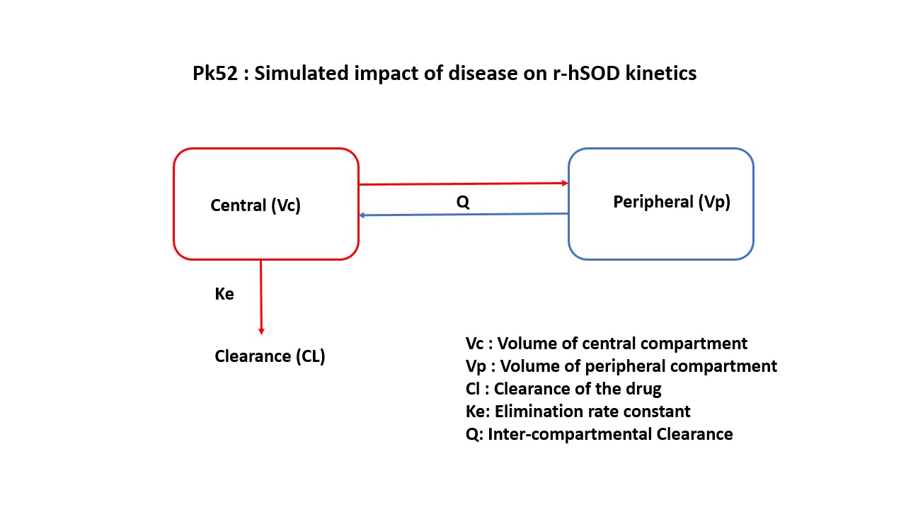
PK52 - Simulated impact of disease on r-hSOD kinetics
1 Background
- Structural model - IV infusion - Two compartment Model
- Route of administration - Rapid intravenous infusion of recombinant human superoxide dismutase (r-hSOD)
- Dosage Regimen - 20 mg/kg IV rapid infusion for 15 seconds in two categories of rats
- Number of Subjects - 1 normal rat, 1 clamped (nephrectomized) rat
In this model, a collection of plasma concentration data of parent drug and concentration of parent and metabolite in urine, will help derive the following parameters: Clearance, Volume of Distribution, Km, Vmax.
2 Learning Outcome
This exercise demonstrates
- The influence of the kidney’s removal on clearance and volume of the central compartment. The effective half life has been increased from 10 mins in normal rats to 90 mins in nephrectomized rats.
- The time to steady state might differ ninefold between the two groups.
- Importance of kidneys in the elimination of r-hSOD and the impact of kidney disease/nephrectomy on the overall kinetics of the drug.
3 Objectives
To build a simple two compartment model with 2 sets of parameters corresponding to normal and clamped rats, simulate the model for clamped versus normal subject and supsequently perform simulation for a population.
4 Libraries
Load the necessary libraries.
5 Model Definition
Note the expression of the model parameters with helpful comments. The model is expressed with differential equations. Residual variability is a proportional error model.
pk_52 = @model begin
    @metadata begin
        desc = "Two Compartment Model"
        timeu = u"minute"
    end

    @param begin
        """
        Clearance (mL/min/kg)
        """
        tvcl ∈ RealDomain(lower = 0)
        """
        Volume of Central Compartment (mL/min/kg)
        """
        tvvc ∈ RealDomain(lower = 0)
        """
        Volume of Peripheral Compartment (mL/min/kg)
        """
        tvvp ∈ RealDomain(lower = 0)
        """
        Intercompartmental Clearance (mL/min/kg)
        """
        tvcld ∈ RealDomain(lower = 0)
        Ω ∈ PDiagDomain(4)
        σ²_prop ∈ RealDomain(lower = 0)
    end

    @random begin
        η ~ MvNormal(Ω)
    end

    @pre begin
        Cl = tvcl * exp(η[1])
        Vc = tvvc * exp(η[2])
        Vp = tvvp * exp(η[3])
        Cld = tvcld * exp(η[4])
    end

    @dynamics begin
        Central' = -(Cl / Vc) * Central - (Cld / Vc) * Central + (Cld / Vp) * Peripheral
        Peripheral' = (Cld / Vc) * Central - (Cld / Vp) * Peripheral
    end

    @derived begin
        cp = @. Central / Vc
        """
        Observed Concentration (μg/mL)
        """
        dv ~ ProportionalNormal.(cp, sqrt(σ²_prop))
    end
end
┌ Warning: Variable `cp` is defined in the `@derived` block using `=` and hence `cp` is not used for model fitting but only returned when simulating: │ If `cp` is a random variable, it must be defined in the `@derived` block using `~`; │ if `cp` should be returned when simulating, it should be defined in the `@observed` block using `=`; │ if `cp` is an intermediate quantity that should not be returned when simulating, it should be defined using `:=`. └ @ Pumas ~/run/_work/PumasTutorials.jl/PumasTutorials.jl/custom_julia_depot/packages/Pumas/GZeMg/src/dsl/model_macro.jl:2351
PumasModel
  Parameters: tvcl, tvvc, tvvp, tvcld, Ω, σ²_prop
  Random effects: η
  Covariates:
  Dynamical system variables: Central, Peripheral
  Dynamical system type: Matrix exponential
  Derived: cp, dv
  Observed: cp, dv
6 Initial Estimates of Model Parameters
The model parameters for simulation are the following. Note that tv represents the typical value for parameters.
tvcl- Clearance (mL/min/kg)tvvc- Volume of Central Compartment (mL/min/kg)tvvp- Volume of Peripheral CompartmentRenal (mL/min/kg)tq- Intercompartmental Clearance (mL/min/kg)Ω- Between Subject Variabilityσ- Residual errors
param1 = (;
    tvcl = 3.0,
    tvvc = 31,
    tvvp = 15,
    tvcld = 0.12,
    Ω = Diagonal([0.01, 0.01, 0.01, 0.01]),
    σ²_prop = 0.04,
)
param2 = (;
tvcl = 0.22,
tvvc = 16,
tvvp = 13,
tvcld = 0.09,
Ω = Diagonal([0.01, 0.01, 0.01, 0.01]),
σ²_prop = 0.04,
)param = vcat(param1, param2)7 Dosage Regimen
A dose of 20 mg/kg to a single rat of 2 categories (normal and clamped)
ev1 = DosageRegimen(20000, cmt = 1)1×10 DataFrame
| Row | time | cmt | amt | evid | ii | addl | rate | duration | ss | route |
|---|---|---|---|---|---|---|---|---|---|---|
| Float64 | Int64 | Float64 | Int8 | Float64 | Int64 | Float64 | Float64 | Int8 | NCA.Route | |
| 1 | 0.0 | 1 | 20000.0 | 1 | 0.0 | 0 | 0.0 | 0.0 | 0 | NullRoute |
8 Single-individual that receives the defined dose
sub1 = Subject(id = "Normal Rat", events = ev1, covariates = (Rat = "Normal_Rat",))Subject
ID: Normal Rat
Events: 1
Covariates: Ratsub2 = Subject(id = "Clamped Rat", events = ev1, covariates = (Rat = "Clamped_Rat",))Subject
ID: Clamped Rat
Events: 1
Covariates: Ratpop2_sub = [sub1, sub2]Population
Subjects: 2
Covariates: Rat
Observations: 9 Single-Subject Simulation
Simulate the plasma concentration after the IV infusion
Initialize the random number generator with a seed for reproducibility of the simulation.
Random.seed!(123)Define the timepoints at which concentration values will be simulated.
sim_pop2_sub = map(
    ((subject, param),) -> simobs(pk_52, subject, param, obstimes = 0:0.1:500),
    zip(pop2_sub, param),
)
Simulated population (Vector{<:Subject})
Simulated subjects: 2
Simulated variables: cp, dv10 Visualize Results
@chain DataFrame(sim_pop2_sub) begin
    dropmissing(:cp)
    data(_) *
    mapping(:time => "Time (hours)", :cp => "Concentration (μg/L)", color = :id => "") *
    visual(Lines; linewidth = 4)
    draw(;
        figure = (; fontsize = 22),
        axis = (;
            yscale = log10,
            ytickformat = i -> (@. string(round(i; digits = 1))),
            xticks = 0:50:500,
            title = "Simulated impact of disease on r-hSOD kinetics",
        ),
        legend = (; position = :bottom),
    )
end
11 Population Simulation
We perform a population simulation with 16 participants.
This code demonstrates how to write the simulated concentrations to a comma separated file (.csv).
par1 = (;
    tvcl = 3.0,
    tvvc = 31,
    tvvp = 15,
    tvcld = 0.12,
    Ω = Diagonal([0.012, 0.0231, 0.0432, 0.0311]),
    σ²_prop = 0.04,
)

par2 = (;
    tvcl = 0.22,
    tvvc = 16,
    tvvp = 13,
    tvcld = 0.09,
    Ω = Diagonal([0.0231, 0.0432, 0.0121, 0.0331]),
    σ²_prop = 0.04,
)

par = vcat(par1, par2)

ev1 = DosageRegimen(20000, cmt = 1)
pop1 = map(i -> Subject(id = i, events = ev1, covariates = (Rat = "Normal_Rat",)), 1:8)
pop2 = map(i -> Subject(id = i, events = ev1, covariates = (Rat = "Clamped_Rat",)), 9:16)
pop = [pop1, pop2]

Random.seed!(1234)
sim_pop = reduce(
    vcat,
    map(
        ((subject, paramᵢ),) -> simobs(
            pk_52,
            subject,
            paramᵢ,
            obstimes = [0.2, 2.1, 4.9, 9.5, 14.7, 29, 60, 119, 239, 480],
        ),
        zip(pop, par),
    ),
)

df_sim = vcat(DataFrame.(sim_pop)...)
#CSV.write("pk_52_sim.csv", df_sim)
12 Conclusion
This tutorial showed how to build a simple two compartment model with 2 sets of parameters corresponding to normal and clamped rats and perform a single subject and a population simulation.