PK53 - Linear antibody kinetics of a two compartment turnover model

1 Background

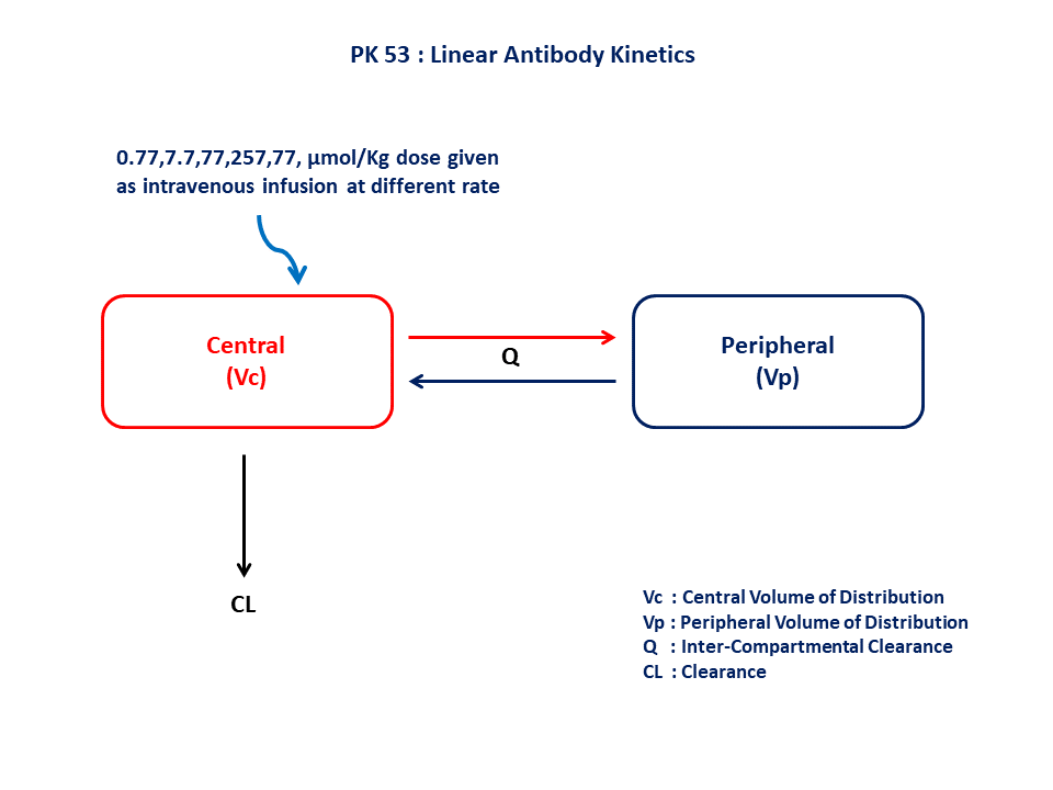
Structural model - Two compartment model
Route of administration - Intravenous infusion
Dosage Regimen - 0.77, 7.7, 77, 257, and 771 μmol/kg dose given as an intravenous infusion
Number of Subjects - 1 (Monkey)

2 Learning Outcome

This exercise demonstrates simulating linear antibody kinetics of different doses of an IV infusion from a two compartment turnover model.

3 Objectives

To build a two-compartment turnover model to characterize linear antibody kinetics, simulate the model for a single subject given different IV dosage regimens, and subsequently perform a simulation for a population.

4 Libraries

Load the necessary libraries.

using PumasUtilities
using Random
using Pumas
using CairoMakie
using AlgebraOfGraphics
using CSV
using DataFramesMeta
using Dates

5 Model Definition

Note the expression of the model parameters with helpful comments. The model is expressed with differential equations. Residual variability is a proportional error model.

In this model, we administer the dose in the central compartment.

pk_53 = @model begin
    @metadata begin
        desc = "Two Compartment Model"
        timeu = u"hr"
    end

    @param begin
        """
        Volume of Central Compartment (L/kg)
        """
        tvvc ∈ RealDomain(lower = 0)
        """
        Volume of Peripheral Compartment (L/kg)
        """
        tvvp ∈ RealDomain(lower = 0)
        """
        Clearance (L/hr/kg)
        """
        tvcl ∈ RealDomain(lower = 0)
        """
        Intercompartmental CLearance (L/hr/kg)
        """
        tvq ∈ RealDomain(lower = 0)
        Ω ∈ PDiagDomain(4)
        """
        Proportional RUV
        """
        σ²_prop ∈ RealDomain(lower = 0)
    end

    @random begin
        η ~ MvNormal(Ω)
    end

    @pre begin
        Vc = tvvc * exp(η[1])
        Vp = tvvp * exp(η[2])
        CL = tvcl * exp(η[3])
        Q = tvq * exp(η[4])
    end

    @dynamics begin
        Central' = -(Q / Vc) * Central + (Q / Vp) * Peripheral - (CL / Vc) * Central
        Peripheral' = (Q / Vc) * Central - (Q / Vp) * Peripheral
    end

    @derived begin
        cp = @. Central / Vc
        """
        Observed Concentration (μM)
        """
        dv ~ @. Normal(cp, sqrt(cp^2 * σ²_prop))
    end
end

PumasModel
  Parameters: tvvc, tvvp, tvcl, tvq, Ω, σ²_prop
  Random effects: η
  Covariates: 
  Dynamical system variables: Central, Peripheral
  Dynamical system type: Matrix exponential
  Derived: cp, dv
  Observed: cp, dv

6 Initial Estimates of Model Parameters

The model parameters for simulation are the following. Note that tv represents the typical value for parameters.

Cl - Clearance (L/hr/kg)
Vc - Volume of Central Compartment (L/kg)
Vp - Volume of Peripheral Compartment (L/kg)
Q - Intercompartmental Clearance (L/hr/kg)
Ω - Between Subject Variability
σ - Residual error

param = (;
    tvvc = 2.139,
    tvvp = 1.5858,
    tvcl = 0.00541,
    tvq = 0.01640,
    Ω = Diagonal([0.01, 0.01, 0.01, 0.01]),
    σ²_prop = 0.04,
)

7 Dosage Regimen

Dose 1: 0.77 μmol/kg given as an IV-infusion at time = 0
Dose 2: 7.7 μmol/kg given as an IV-infusion at time = 72.17
Dose 3: 77 μmol/kg given as an IV-infusion at time = 144.17
Dose 4: 257 μmol/kg given as an IV-infusion at time = 216.6
Dose 5: 771 μmol/kg given as an IV-infusion at time = 288.52

ev1 = DosageRegimen(0.77, time = 0, cmt = 1, duration = 0.416667)

1×10 DataFrame

Row	time	cmt	amt	evid	ii	addl	rate	duration	ss	route
	Float64	Int64	Float64	Int8	Float64	Int64	Float64	Float64	Int8	NCA.Route
1	0.0	1	0.77	1	0.0	0	1.848	0.416667	0	NullRoute

ev2 = DosageRegimen(7.7, time = 72.17, cmt = 1, duration = 0.5)

1×10 DataFrame

Row	time	cmt	amt	evid	ii	addl	rate	duration	ss	route
	Float64	Int64	Float64	Int8	Float64	Int64	Float64	Float64	Int8	NCA.Route
1	72.17	1	7.7	1	0.0	0	15.4	0.5	0	NullRoute

ev3 = DosageRegimen(77, time = 144.17, cmt = 1, duration = 0.5)

1×10 DataFrame

Row	time	cmt	amt	evid	ii	addl	rate	duration	ss	route
	Float64	Int64	Float64	Int8	Float64	Int64	Float64	Float64	Int8	NCA.Route
1	144.17	1	77.0	1	0.0	0	154.0	0.5	0	NullRoute

ev4 = DosageRegimen(257, time = 216.6, cmt = 1, duration = 0.4)

1×10 DataFrame

Row	time	cmt	amt	evid	ii	addl	rate	duration	ss	route
	Float64	Int64	Float64	Int8	Float64	Int64	Float64	Float64	Int8	NCA.Route
1	216.6	1	257.0	1	0.0	0	642.5	0.4	0	NullRoute

ev5 = DosageRegimen(771, time = 288.52, cmt = 1, duration = 0.5)

1×10 DataFrame

Row	time	cmt	amt	evid	ii	addl	rate	duration	ss	route
	Float64	Int64	Float64	Int8	Float64	Int64	Float64	Float64	Int8	NCA.Route
1	288.52	1	771.0	1	0.0	0	1542.0	0.5	0	NullRoute

ev = DosageRegimen(ev1, ev2, ev3, ev4, ev5)

5×10 DataFrame

Row	time	cmt	amt	evid	ii	addl	rate	duration	ss	route
	Float64	Int64	Float64	Int8	Float64	Int64	Float64	Float64	Int8	NCA.Route
1	0.0	1	0.77	1	0.0	0	1.848	0.416667	0	NullRoute
2	72.17	1	7.7	1	0.0	0	15.4	0.5	0	NullRoute
3	144.17	1	77.0	1	0.0	0	154.0	0.5	0	NullRoute
4	216.6	1	257.0	1	0.0	0	642.5	0.4	0	NullRoute
5	288.52	1	771.0	1	0.0	0	1542.0	0.5	0	NullRoute

8 Single-individual that receives the defined dose

sub1 = Subject(id = 1, events = ev)

Subject
  ID: 1
  Events: 10

9 Single-Subject Simulation

Simulate for plasma concentration with the specific observation time points after the intravenous administration.

Initialize the random number generator with a seed for reproducibility of the simulation.

Random.seed!(123)

Define the timepoints at which concentration values will be simulated.

sim_sub1 = simobs(pk_53, sub1, param, obstimes = 0.01:0.01:2000)

SimulatedObservations
  Simulated variables: cp, dv
  Time: 0.01:0.01:2000.0

df1 = DataFrame(sim_sub1)
first(df1, 5)

5×22 DataFrame

Row	id	time	cp	dv	evid	amt	cmt	rate	duration	ss	ii	route	η_1	η_2	η_3	η_4	Central	Peripheral	Vc	Vp	CL	Q
	String?	Float64	Float64?	Float64?	Int64?	Float64?	Symbol?	Float64?	Float64?	Int8?	Float64?	NCA.Route?	Float64?	Float64?	Float64?	Float64?	Float64?	Float64?	Float64?	Float64?	Float64?	Float64?
1	1	0.0	missing	missing	1	0.77	Central	1.848	0.416667	0	0.0	NullRoute	-0.0494927	0.029404	0.114707	-0.0522506	missing	missing	2.03571	1.63312	0.00606756	0.0155651
2	1	0.01	0.00907741	0.0132313	0	missing	missing	missing	missing	missing	missing	missing	-0.0494927	0.029404	0.114707	-0.0522506	0.018479	7.06444e-7	2.03571	1.63312	0.00606756	0.0155651
3	1	0.02	0.0181539	0.012376	0	missing	missing	missing	missing	missing	missing	missing	-0.0494927	0.029404	0.114707	-0.0522506	0.036956	2.82559e-6	2.03571	1.63312	0.00606756	0.0155651
4	1	0.03	0.0272294	0.0261162	0	missing	missing	missing	missing	missing	missing	missing	-0.0494927	0.029404	0.114707	-0.0522506	0.0554311	6.35714e-6	2.03571	1.63312	0.00606756	0.0155651
5	1	0.04	0.0363039	0.0431697	0	missing	missing	missing	missing	missing	missing	missing	-0.0494927	0.029404	0.114707	-0.0522506	0.0739042	1.13008e-5	2.03571	1.63312	0.00606756	0.0155651

10 Visualize Results

@chain DataFrame(sim_sub1) begin
    dropmissing(:cp)
    data(_) *
    mapping(:time => "Time (hours)", :cp => "Concentration (μM)") *
    visual(Lines; linewidth = 4)
    draw(;
        figure = (; fontsize = 22),
        axis = (;
            yscale = log10,
            ytickformat = i -> (@. string(round(i; digits = 1))),
            xticks = 0:200:2000,
        ),
    )
end

11 Population Simulation

We perform a population simulation with 48 participants, and simulate concentration values for 72 hours following 6 doses administered every 8 hours.

This code demonstrates how to write the simulated concentrations to a comma separated file (.csv).

par = (;
    tvvc = 2.139,
    tvvp = 1.5858,
    tvcl = 0.0054,
    tvq = 0.01653,
    Ω = Diagonal([0.045, 0.024, 0.012, 0.0224]),
    σ²_prop = 0.04,
)
ev = DosageRegimen(ev1, ev2, ev3, ev4, ev5)
pop = map(i -> Subject(id = i, events = ev), 1:50)

Random.seed!(1234)
sim_pop = simobs(
    pk_53,
    pop,
    par,
    obstimes = [
        72.67,
        74.17,
        78.17,
        84.17,
        96.17,
        120.17,
        144.17,
        144.67,
        146.17,
        150.17,
        156.17,
        168.17,
        192.17,
        216.17,
        217,
        218.5,
        222.5,
        228.5,
        240.5,
        264.5,
        288.5,
        289.02,
        290.5,
        294.5,
        300.5,
        312.5,
        336.5,
        360.5,
        483.92,
        651.25,
        983.92,
        1751.92,
    ],
)

pkdata_53_sim = DataFrame(sim_pop)
#CSV.write("pk_53_sim.csv", pkdata_53_sim)

12 Conclusion

This tutorial showed how to build a two compartment turnover model to characterize linear antibody kinetics and perform a single subject and a population simulation.