using Pumas
using PumasUtilities
using CairoMakie
using AlgebraOfGraphics
using DataFramesMeta
Modeling Tumor Growth and Therapeutic Response
1 Introduction
Understanding tumor growth and its inhibition by therapeutic agents is fundamental to optimizing cancer treatment strategies. Mathematical models of tumor growth inhibition (TGI) provide a quantitative framework for integrating experimental and clinical data to simulate tumor dynamics, predict treatment outcomes, and inform drug development decisions. These models are also referred to as tumor growth dynamics (TGD) models in some contexts.
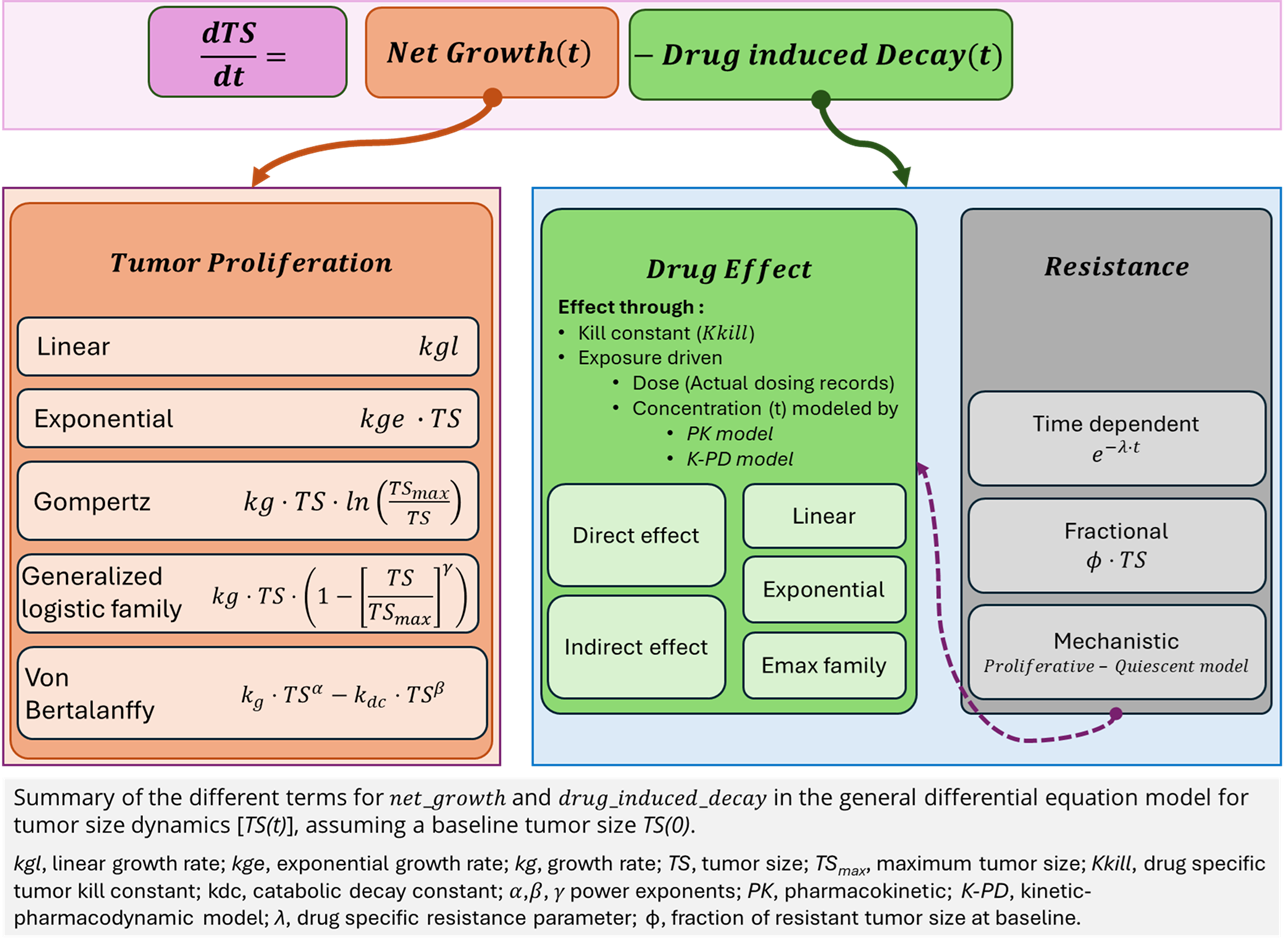
Tumor dynamics can be broadly described as a balance between growth and decay (Figure 1), often represented mathematically as:
\(\frac{dTS}{dt} = Growth(t) - Decay(t)\)
Where 𝑇𝑆(𝑡) represents the tumor size at time 𝑡. Different models vary in how they define the growth and decay components, depending on the underlying biology and drug mechanisms.
Figure 1: Overview of TGI Model Framework
1.0.1 Tumor Size Measurements and RECIST Criteria
In clinical studies, tumor burden is typically quantified using imaging-based measurements. The most common metric is the Sum of Longest Diameters (SLD) across a set of target lesions, as defined by the RECIST (Response Evaluation Criteria In Solid Tumors) guidelines (Eisenhauer et al. 2009). Alternatively, some studies use the Sum of Product of Diameters (SPD). These continuous measurements form the basis for categorical RECIST responses:
CR(Complete Response): Disappearance of all target lesionsPR(Partial Response): ≥30% decrease in SLD from baselinePD(Progressive Disease): ≥20% increase in SLD, or appearance of new lesionsSD(Stable Disease): Neither sufficient shrinkage for PR nor growth for PD
TGI models are commonly fit to SLD or SPD trajectories to predict response dynamics and explore time-to-event endpoints like Time to Progression (TTP), Progression-Free Survival (PFS) or Overall Survival (OS).
This tutorial presents a comprehensive overview of commonly used tumor growth models and treatment effect models, implemented in Pumas. It follows a modular structure:
1.0.2 Typical Growth Models
Tumor Growth functions characterize how tumors proliferate over time in absence of treatment. Each model captures different biological assumptions:
- Linear: No saturation, constant growth rate
- Exponential: No saturation, growth rate proportional to tumor size
- Logistic and Generalized logistic: Growth saturates as tumor approaches carrying capacity
- Gompertz: Intermediate between exponential and logistic
- Power-law / von Bertalanffy: More flexibility in growth kinetics
1.0.3 Typical treatment effect models
Drug Effect models help to understand how a drug impacts tumor size. Tumor shrinkage or inhibition is modeled through:
- Direct Effects: Linear or Emax-type kill functions
- Indirect Effects: Models with intermediate signaling or delayed responses
- K-PD Models: When PK data is unavailable, drug effect is modeled empirically
1.0.4 Typical resistance models
Resistance may develop over long-term treatment and can be described as:
- Time-dependent: Gradual reduction in drug effect
- Fractional: Presence of resistant subpopulations from baseline
- Mechanistic frameworks : Proliferative–Quiescent (P–Q)
1.0.5 Applications of TGI Modeling
TGI models are used to:
- Simulate tumor dynamics under various treatment regimens
- Predict time to progression or relapse
- Support regulatory submissions and dose justification
- Explore new therapeutic strategies including immunotherapy and combinations
📊 Each section includes the mathematical formulation, model code, and simulated outputs to promote a deep understanding of the models and their assumptions. We explore these models using single-subject simulations to compare their growth behaviors in the absence of treatment. By default, inter-individual variability (IIV) is set to zero to illustrate typical dynamics; increasing IIV allows for population-level simulations that capture variability across subjects.
2 Tumor Growth Models
2.1 Introduction
Tumor growth models aim to characterize how a tumor expands over time in the absence of treatment. These models form the backbone of TGI frameworks and differ mainly in how they describe the proliferation dynamics.
We denote the tumor size at time 𝑡 as 𝑇𝑆(𝑡) and the initial tumor size at time 0 as 𝑇𝑆0. The rate of change of tumor size is governed by a growth law of the form:
\(TS(0) = TS0\)
\(\frac{dTS}{dt} = Growth(t)\)
Each model differs in the specific mathematical formulation of the growth function. The choice of model depends on biological plausibility, data support, and computational tractability. Below, we introduce several widely-used models:
Linear Growth: Constant increase over time
Exponential Growth: Proportional to current size
Gompertz Growth: Slows down exponentially with time
Logistic and Generalized Logistic Growth: Incorporates carrying capacity
Power-Law and von Bertalanffy Models: Size-dependent, mechanistically interpretable
In subsequent sections, we will explore each of these models in detail, simulate tumor growth trajectories, and compare their predictions under consistent initial conditions.
Baseline tumor size (\(TS0\)) modeling can be approached in different ways—such as fixing it to the observed value, estimating it as an individual-specific parameter, or combining both observed and estimated components. In this tutorial, we follow the common and preferred approach of estimating \(TS0\) as an individual-specific parameter with interindividual variability (B1 method, Dansirikul, Silber, and Karlsson (2008)).
2.2 Linear Tumor Growth Model
The linear tumor growth model assumes that the tumor increases in size at a constant (zero order) rate, regardless of its current size/volume. This may be a reasonable approximation for early tumor development or slow-growing tumors.
Model Equation
The linear growth equation is defined as:
\(TS(0) = TS0\)
\(\frac{dTS}{dt} = k_{gl}\)
Where:
𝑇𝑆0is the tumor size at time0,𝑘𝑔lis the constant growth rate.
The analytical solution of this growth function can be written as:
\(𝑇𝑆(𝑡) = TS0 + k_{gl} \cdot t\)
Where 𝑇𝑆(𝑡) is the tumor size at time 𝑡 and 𝑇𝑆0 is the initial tumor size at time 0.
Note
For linear differential equations like the linear tumor growth model, Pumas automatically detects linearity and uses the analytical solution internally for more efficient simulation. This behavior can be disabled using checklinear = false in the @options block if needed.
Here is an example of linear tumor growth model using Pumas.
Load the necessary libraries to get started.
The linear tumor growth model is defined as follows:
linear_model = @model begin
    @metadata begin
        desc = "linear tumor growth  model"
        timeu = u"d"
    end

    @param begin
        """
        Linear tumor growth rate (kgl; mm/day)
        """
        tvkgl ∈ RealDomain(; lower = 0)
        """
        Baseline tumor size (TS0; mm)
        """
        tvTS0 ∈ RealDomain(; lower = 0)

        # Inter-individual variability
        """
          - Ωkgl
          - ΩTS0
        """
        Ω ∈ PDiagDomain(2)

        # Residual variability
        """
        Additive residual error
        """
        σ ∈ RealDomain(; lower = 0)
    end

    @random begin
        η ~ MvNormal(Ω)
    end

    @init TS = TS0

    @pre begin
        kgl = tvkgl * exp(η[1])
        TS0 = tvTS0 * exp(η[2])
    end

    @dynamics begin
        TS' = kgl
    end

    @derived begin
        tumor_size ~ Normal.(TS, σ)
    end
end;
The initial estimates of the linear tumor growth model parameters are:
tvkgl- Linear tumor growth ratetvTS0- Tumor size at time 0Ω- Between subject variabilityσ- Residual error
linear_params = (; tvkgl = 45.33, tvTS0 = 700, Ω = Diagonal([0, 0]), σ = 0);The simulation for the linear tumor growth model is performed as follows:
linear_sim = simobs(linear_model, Subject(), linear_params; obstimes = 0:1:100);The results of the linear tumor growth model are visualized as follows:
Show code
# convert simulated data into a dataframe
sim_df = DataFrame(linear_sim);

# select only evid = 0 rows (observations only)
plot_df = filter(row -> (row.evid == 0), sim_df)

# plotting tumor size vs time
plt_lin = data(plot_df) * mapping(:time, :tumor_size) * visual(Lines, linewidth = 2)

# Define tick positions based on your max time
xtick_vals = 0:30:maximum(plot_df.time)

# Updating title and axis names
fig = draw(
    plt_lin;
    axis = (;
        title = "Linear Tumor Growth Model",
        xlabel = "Time (days)",
        ylabel = "Tumor Size",
        xticks = xtick_vals,
    ),
    figure = (size = (650, 500),),
)

# Print output
fig
2.3 Exponential Tumor Growth Model
The exponential growth model assumes that the tumor expands at a rate proportional to its current size, resulting in non-saturable, continuous growth over time. This model is commonly used to describe fast-growing tumors, particularly in early-stage disease or in the absence of resource limitations such as nutrients or oxygen. One of the earlier applications of the exponential growth model was in colorectal cancer, where it was used to characterize tumor progression (Claret et al. 2009).
Model Equation
The exponential growth equation is defined as:
\(TS(0) = TS0\)
\(\frac{dTS}{dt} = k_{ge} \cdot TS(t)\)
Where:
𝑇𝑆0is the tumor size at time0,𝑘𝑔eis the exponential growth rate.
The analytical solution of this growth function can be written as:
\(𝑇𝑆(𝑡) = TS0 \cdot e^{k_{ge} \cdot t}\)
This model leads to unbounded growth and does not account for saturation or carrying capacity.
Here is an example of an exponential tumor growth model development using Pumas.
Load the necessary libraries to get started.
using Pumas
using PumasUtilities
using CairoMakie
using AlgebraOfGraphics
The exponential tumor growth model is defined as follows:
exponential_model = @model begin
    @metadata begin
        desc = "exponential tumor growth  model"
        timeu = u"d"
    end
    @param begin
        """
        Exponential tumor growth rate (kge; /day)
        """
        tvkge ∈ RealDomain(; lower = 0)
        """
        Baseline tumor size (TS0; mm)
        """
        tvTS0 ∈ RealDomain(; lower = 0)

        # Inter-individual variability
        """
          - Ωkgl
          - ΩTS0
        """
        Ω ∈ PDiagDomain(2)

        # Residual variability
        """
        Additive residual error
        """
        σ ∈ RealDomain(; lower = 0)
    end
    @random begin
        η ~ MvNormal(Ω)
    end
    @init TS = TS0

    @pre begin
        kge = tvkge * exp(η[1])
        TS0 = tvTS0 * exp(η[2])
    end
    @dynamics begin
        TS' = kge * TS
    end

    @derived begin
        tumor_size ~ Normal.(TS, σ)
    end
end;
The initial estimates of the exponential tumor growth model parameters are:
tvkge- exponential tumor growth ratetvTS0- tumor size at time 0Ω- Between Subject Variabilityσ- Residual error
exponential_params = (; tvkge = 0.029, tvTS0 = 700, Ω = Diagonal([0, 0]), σ = 0);The simulation for the exponential tumor growth model is performed as follows:
exponential_sim =
    simobs(exponential_model, Subject(), exponential_params; obstimes = 0:1:100);
The results of the exponential tumor growth model are visualized as follows:
Show code
# convert simulated data into a dataframe
sim_df = DataFrame(exponential_sim);

# select only evid = 0 rows (observations only)
plot_df = filter(row -> (row.evid == 0), sim_df)

# plotting tumor size vs time
plt_lin = data(plot_df) * mapping(:time, :tumor_size) * visual(Lines, linewidth = 2)

# Define tick positions based on your max time
xtick_vals = 0:30:maximum(plot_df.time)

# Updating title and axis names
fig = draw(
    plt_lin;
    axis = (;
        title = "Exponential Growth Model",
        xlabel = "Time (days)",
        ylabel = "Tumor Size",
        xticks = xtick_vals,
    ),
    figure = (size = (650, 500),),
)

# Print output
fig
2.4 Exponential-Linear Tumor Growth Model
The exponential-linear model captures biphasic tumor growth: an initial exponential phase (rapid cell division) followed by a linear phase (growth slows due to resource limitations or necrosis). This hybrid model is often more realistic for preclinical tumor data. A clinical application of this model is described in the work by Ouerdani et al. (2016).
Model Equation
The exponential-linear tumor growth model dynamics are expressed as follows:
\(TS(0) = TS0\)
\(\frac{dTS}{dt} = k_{ge} \cdot TS, \, t \leq \tau\)
\(\frac{dTS}{dt} = k_{gl}, \, t > \tau\)
Where:
𝑇𝑆0is the tumor size at time0,𝑘𝑔eis the exponential growth rate,𝑘𝑔lis the constant growth rate.
The transition time from the exponential phase to the linear phase is defined as follows:
\(\tau = \frac{1}{k_{ge}} \ln(\frac{k_{gl}}{k_{ge} \cdot TS0})\)
The analytical solution of this growth function can be written as:
\(TS = TS0 \cdot e^{k_{ge} \cdot t}, \, t \leq \tau\)
\(TS = k_{gl} \cdot (t - \tau) + TS0 \cdot e^{k_{ge} \cdot \tau}, \, t > \tau\)
Here is an example of an exponential-linear tumor growth model using Pumas.
Load the necessary libraries to get started.
using Pumas
using PumasUtilities
using CairoMakie
using AlgebraOfGraphics
The exponential-linear tumor growth model is defined as follows:
exp_lin_model = @model begin
    @metadata begin
        desc = "exponential linear tumor growth  model"
        timeu = u"d"
    end
    @param begin
        """
        Linear tumor growth rate (kgl; mm/day)
        """
        tvkgl ∈ RealDomain(; lower = 0)
        """
        Exponential tumor growth rate (kge; /day)
        """
        tvkge ∈ RealDomain(; lower = 0)
        """
        Baseline tumor size (TS0; mm)
        """
        tvTS0 ∈ RealDomain(; lower = 0)

        # Inter-individual variability
        """
          - Ωkgl
          - Ωkge
          - ΩTS0
        """
        Ω ∈ PDiagDomain(3)

        # Residual variability
        """
        Additive residual error
        """
        σ ∈ RealDomain(; lower = 0)

    end
    @random begin
        η ~ MvNormal(Ω)
    end
    @init TS = TS0

    @pre begin
        kgl = tvkgl * exp(η[1])
        kge = tvkge * exp(η[2])
        TS0 = tvTS0 * exp(η[3])

        # transition time from the exponential phase to the linear phase
        τ = (1 / kge) * log(kgl / (kge * TS0))
        flg = t <= τ ? 1 : 0
    end
    @dynamics begin
        TS' = kge * TS * (flg) + kgl * (1 - flg)
    end
    @derived begin
        tumor_size ~ Normal.(TS, σ)
    end
end;
The initial estimates of the exponential-linear tumor growth model parameters are:
tvkgl- Linear tumor growth ratetvkge- Exponential tumor growth ratetvTS0- Tumor size at time 0Ω- Between subject variabilityσ- Residual error
exp_lin_params =
    (; tvkgl = 40.33, tvkge = 0.02, tvTS0 = 700, Ω = Diagonal([0, 0, 0]), σ = 0);
The simulation for the exponential-linear tumor growth model is performed as follows:
exp_lin_sim = simobs(exp_lin_model, Subject(), exp_lin_params; obstimes = 0:1:100);The results of the exponential-linear tumor growth model are visualized as follows:
Show code
# convert simulated data into a dataframe
sim_df = DataFrame(exp_lin_sim);

# select only evid = 0 rows (observations only)
plot_df = filter(row -> (row.evid == 0), sim_df)

# plotting tumor size vs time
plt_lin = data(plot_df) * mapping(:time, :tumor_size) * visual(Lines, linewidth = 2)

# Define tick positions based on your max time
xtick_vals = 0:30:maximum(plot_df.time)

# Updating title and axis names
fig = draw(
    plt_lin;
    axis = (;
        title = "Exponential-linear Tumor Growth Model",
        xlabel = "Time (days)",
        ylabel = "Tumor Size",
        xticks = xtick_vals,
    ),
    figure = (size = (650, 500),),
)

# Print output
fig
2.5 Gompertz Tumor Growth Model
The Gompertz model assumes that the tumor growth rate decreases exponentially over time. It captures the rapid initial growth and gradual saturation often observed in experimental and clinical tumor data (Belfatto et al. 2016).
The model is a generalization of the logistic model with a sigmoidal curve that is asymmetrical with the point of inflection. The curve was eventually applied to model growth in size of entire organisms.
Model Equation
This model is based on the well-known Gompertz function, commonly used to model systems that experience saturation for large values in the dependent variable:
\(TS(0) = TS0\)
\(\frac{dTS}{dt} = TS \cdot \beta \cdot \ln(\frac{TS_{max}}{TS})\)
Where:
𝑇𝑆0is the tumor size at time0,𝑘𝑔eis the tumor growth rate,tvTSmxis the maximum tumor size.
The analytical solution of this growth function can be written as:
\(TS = TS_{max} \cdot e^{e^{-\beta \cdot t} \cdot \ln(\frac{TS0}{TS_{max}})}\)
This form of the analytical solution clearly shows that the Gompertz function is being used. A more concise formulation is provided below for improved readability and clarity.
\(TS = TS_{max} \cdot (\frac{TS0}{TS_{max}})^{e^{-\beta \cdot t}}\)
Here is an example of a Gompertz tumor growth model using Pumas.
Load the necessary libraries to get started.
using Pumas
using PumasUtilities
using CairoMakie
using AlgebraOfGraphics
The Gompertz tumor growth model is defined as follows:
gompertz_model = @model begin
    @metadata begin
        desc = "Gompertz tumor growth model"
        timeu = u"d"
    end

    @param begin
        """
        Tumor growth rate (β; /day)
        """
        tvβ ∈ RealDomain(; lower = 0)
        """
        Baseline tumor size (TS0; mm)
        """
        tvTS0 ∈ RealDomain(; lower = 0)
        """
        Maximum tumor size (TSmax; mm)
        """
        tvTSmax ∈ RealDomain(; lower = 0)

        # Inter-individual variability
        """
          - Ωβ
          - ΩTS0
          - ΩTSmax
        """
        Ω ∈ PDiagDomain(3)

        # Residual variability
        """
        Additive residual error
        """
        σ ∈ RealDomain(; lower = 0)
    end
    @random begin
        η ~ MvNormal(Ω)
    end
    @init TS = TS0

    @pre begin
        β = tvβ * exp(η[1])
        TS0 = tvTS0 * exp(η[2])
        TSmax = tvTSmax * exp(η[3])
    end
    @dynamics begin
        TS' = TS * β * log(TSmax / TS)
    end
    @derived begin
        tumor_size ~ Normal.(TS, σ)
    end
end;
The initial estimates of the Gompertz tumor growth model parameters are:
tvβ- Tumor growth ratetvTS0- Tumor size at time 0tvTSmx- Maximum tumor sizeΩ- Between subject variabilityσ- Residual error
gompertz_params =
    (; tvβ = 0.08, tvTS0 = 700, tvTSmax = 5_000, Ω = Diagonal([0, 0, 0]), σ = 0);
The simulation for the Gompertz tumor growth model is performed as follows:
gompertz_sim = simobs(gompertz_model, Subject(), gompertz_params; obstimes = 0:1:100);The results of the Gompertz tumor growth model are visualized as follows:
Show code
# convert simulated data into a dataframe
sim_df = DataFrame(gompertz_sim);

# select only evid = 0 rows (observations only)
plot_df = filter(row -> (row.evid == 0), sim_df)

# plotting tumor size vs time
plt_lin = data(plot_df) * mapping(:time, :tumor_size) * visual(Lines, linewidth = 2)

# Define tick positions based on your max time
xtick_vals = 0:30:maximum(plot_df.time)

# Updating title and axis names
fig = draw(
    plt_lin;
    axis = (;
        title = "Gompertz Tumor Growth Model",
        xlabel = "Time (days)",
        ylabel = "Tumor Size",
        xticks = xtick_vals,
    ),
    figure = (size = (650, 500),),
)

# Print output
fig
2.6 Logistic and Generalized Logistic Tumor Growth Model
The logistic growth model introduces the concept of a carrying capacity, which represents the maximum tumor size that can be sustained due to limitations in resources such as nutrients, oxygen, and space. As the tumor approaches this limit, the growth rate slows, transitioning from exponential to plateauing behavior. This model is particularly useful for modeling tumors in later stages or under immune and vascular constraints. Clinical and preclinical applications of the logistic model can be found in studies by Ollier et al. (2017) and Ribba et al. (2012).
The generalized logistic model extends the standard logistic framework by introducing a shape parameter, which allows greater flexibility in defining how sharply the tumor transitions from exponential growth to saturation. This model is well-suited to capture a broader spectrum of tumor growth behaviors — including scenarios where growth slows gradually or drops off more abruptly as the tumor approaches its maximum size.
Like the logistic model, it incorporates a carrying capacity that limits unbounded growth, reflecting biological constraints such as nutrient availability, immune response, or spatial limitations. The generalized logistic model produces a characteristic sigmoidal response, where the initial phase resembles exponential growth, followed by a tapering off that depends on the value of the shape parameter. This sigmoidal behavior is particularly useful when tumor size is observed to plateau at varying rates across treatment arms or tumor types.
Compared to linear and exponential models, which imply indefinite growth, both the logistic and generalized logistic models provide a biologically realistic saturation effect and have been effectively applied when the maximum tumor burden is assumed to be fixed — as demonstrated in multiple preclinical and clinical modeling studies.
2.6.1 Logistic Tumor Growth Model
Model Equation
The system’s dynamics have the following form in this case:
\(TS(0) = TS0\)
\(\frac{dTS}{dt} = k_{ge} \cdot TS \cdot (1 - \frac{TS}{TS_{max}})\)
Where:
𝑇𝑆0is the tumor size at time0,𝑘𝑔eis the exponential growth rate,TS_maxrepresents the tumor’s carrying capacity i.e the maximum size that can be reached by the tumor.
It can be shown that this differential equation has the following analytical solution:
\(TS = \frac{TS_{max} \cdot TS0}{TS0 + (TS_{max} - TS0) \cdot e^{-k_{ge} \cdot t}}\)
When logistic models should be used?
Logistic models can simulate the fact that tumor growth is limited by nutritional, immunological or spatial constraints by including a carrying capacity into the model at which the tumor volume plateaus. This carrying capacity is in line with the observation that tumor growth slows down when the tumor volume becomes large.
Why limited carrying capacity?
The carrying capacity can be interpreted to comprise a number of biological constraints to tumor cell proliferation. These constraints include the availability of nutrients and oxygen and thus, the concept of tumor angiogenesis is implicit in the carrying capacity. In addition, the pressure of immune cells attacking tumor cells limits the niche the tumor cells can fill and thus, the concept of antitumor immune response is implicit in the carrying capacity.
Here is an example of a logistic tumor growth model using Pumas.
Load the necessary libraries to get started.
using Pumas
using PumasUtilities
using CairoMakie
using AlgebraOfGraphics
The logistic tumor growth model is defined as follows:
logistic_model = @model begin
    @metadata begin
        desc = "logistic tumor growth  model"
        timeu = u"d"
    end
    @param begin
        """
        Exponential tumor growth rate (kge; /day)
        """
        tvkge ∈ RealDomain(; lower = 0)
        """
        Baseline tumor size (TS0; mm)
        """
        tvTS0 ∈ RealDomain(; lower = 0)
        """
        Maximum tumor size (TSmax; mm)
        """
        tvTSmax ∈ RealDomain(; lower = 0)

        # Inter-individual variability
        """
          - Ωkge
          - ΩTS0
          - ΩTSmax
        """
        Ω ∈ PDiagDomain(3)

        # Residual variability
        """
        Additive residual error
        """
        σ ∈ RealDomain(; lower = 0)
    end
    @random begin
        η ~ MvNormal(Ω)
    end
    @init TS = TS0

    @pre begin
        kge = tvkge * exp(η[1])
        TS0 = tvTS0 * exp(η[2])
        TSmax = tvTSmax * exp(η[3])
    end
    @dynamics begin
        TS' = kge * TS * (1 - TS / TSmax)
    end
    @derived begin
        tumor_size ~ Normal.(TS, σ)
    end
end;
The initial estimates of the logistic tumor growth model parameters are:
tvkge- Tumor growth ratetvTS0- Tumor size at time 0tvTSMAX- Maximum tumor sizeΩ- Between subject variabilityσ- Residual error
logistic_params =
    (; tvkge = 0.07, tvTS0 = 700, tvTSmax = 5_000, Ω = Diagonal([0, 0, 0]), σ = 0);
The simulation for the logistic tumor growth model is performed as follows:
logistic_sim = simobs(logistic_model, Subject(), logistic_params; obstimes = 0:0.1:100);The results of the logistic tumor growth model are visualized as follows:
Show code
sim_df = DataFrame(logistic_sim);

plot_df = filter(row -> (row.evid == 0), sim_df)

plt_lin = data(plot_df) * mapping(:time, :tumor_size) * visual(Lines, linewidth = 2)

# Define tick positions based on your max time
xtick_vals = 0:30:maximum(plot_df.time)

fig = draw(
    plt_lin;
    axis = (;
        title = "Logistic Tumor Growth Model",
        xlabel = "Time (days)",
        ylabel = "Tumor Size",
        xticks = xtick_vals,
    ),
    figure = (size = (650, 500),),
)

fig
2.6.2 Generalized Logistic Tumor Growth Model
This is an extension of the logistic model which produces a response resembling the generalized logistic function.
Model Equation
The differential equation that defines this model has the following form:
\(TS(0) = TS0\)
\(\frac{dTS}{dt} = kge \cdot TS \cdot (1 - (\frac{TS}{TS_{max}})^{\gamma})\)
Note that this model generalizes the logistic model, with
gamma = 1yielding the standard logistic form.
Here’s the analytical solution for this model:
\(TS = \frac{TS_{max} \cdot TS0}{(TS0^{\gamma} + (TS_{max}^{\gamma} - TS0^{\gamma}) \cdot e^{-kge \cdot \gamma \cdot t})^{\frac{1}{\gamma}}}\)
Here is a simple example of generalized logistic tumor growth model development using Pumas.
Load the necessary libraries to get started.
using Pumas
using PumasUtilities
using CairoMakie
using AlgebraOfGraphics
The generalized logistic tumor growth model is defined as follows:
gen_logistic_model = @model begin
    @metadata begin
        desc = "generalized logistic tumor growth  model"
        timeu = u"d"
    end
    @param begin
        """
        Exponential tumor growth rate (kge; /day)
        """
        tvkge ∈ RealDomain(; lower = 0)
        """
        Baseline tumor size (TS0; mm)
        """
        tvTS0 ∈ RealDomain(; lower = 0)
        """
        Maximum tumor size (TSmax; mm)
        """
        tvTSmax ∈ RealDomain(; lower = 0)
        """
        Power coefficient (γ; -)
        """
        tvγ ∈ RealDomain(; lower = 0, upper = 5)

        # Inter-individual variability
        """
          - Ωkge
          - ΩTS0
          - ΩTSmax
          - Ωγ
        """
        Ω ∈ PDiagDomain(4)

        # Residual variability
        """
        Additive residual error
        """
        σ ∈ RealDomain(; lower = 0)
    end
    @random begin
        η ~ MvNormal(Ω)
    end
    @init TS = TS0
    @pre begin
        kge = tvkge * exp(η[1])
        TS0 = tvTS0 * exp(η[2])
        TSmax = tvTSmax * exp(η[3])
        γ = tvγ * exp(η[4])
    end
    @dynamics begin
        TS' = kge * TS * (1 - (TS / TSmax)^γ)
    end
    @derived begin
        tumor_size ~ Normal.(TS, σ)
    end
end;
The initial estimates of the generalized logistic tumor growth model parameters are:
tvkge- Tumor growth ratetvTS0- Tumor size at the beginning of the studytvTSMAX- Maximum tumor sizetvγ- PowerΩ- Between subject variabilityσ- Residual error
gen_logistic_params_1 = (;
    tvkge = 0.06,
    tvTS0 = 700,
    tvTSmax = 5_000,
    tvγ = 0.5,
    Ω = Diagonal([0, 0, 0, 0]),
    σ = 0,
);
Change the gamma value to show the difference [0.5 vs 5.0]
gen_logistic_params_2 = (;
    tvkge = 0.06,
    tvTS0 = 700,
    tvTSmax = 5_000,
    tvγ = 5,
    Ω = Diagonal([0, 0, 0, 0]),
    σ = 0,
);
The simulation for the generalized logistic tumor growth model is performed as follows:
gen_logistic_sim_1 =
    simobs(gen_logistic_model, Subject(), gen_logistic_params_1; obstimes = 0:0.1:100);
gen_logistic_sim_2 =
simobs(gen_logistic_model, Subject(), gen_logistic_params_2; obstimes = 0:0.1:100);The results of the generalized logistic tumor growth model are visualized as follows:
Show code
# ─────────────────────────── tidy helper ─────────────────────────────────
function tidy(simdf::DataFrame, label::String)

    df = copy(simdf)

    # 1. Standardise observable name
    if :ts in names(df) && !(:tumor_size in names(df))
        rename!(df, :ts => :tumor_size)
    end

    # 2. Keep only the columns we care about
    keepcols = intersect(names(df), ["time", "tumor_size"])      # make sure they exist
    df = df[:, keepcols]                                        # drop the rest

    # 3. Add model identifier
    df.model = fill(label, nrow(df))
    return df
end

# ─────────────────────────── build long DF ───────────────────────────────
dfs = [
    tidy(DataFrame(gen_logistic_sim_1), "Gen Logistic (γ = 0.5)"),
    tidy(DataFrame(gen_logistic_sim_2), "Gen Logistic (γ = 5.0)"),
];

df_gen = vcat(dfs...; cols = :union);

# ─────────────────────────── plot ────────────────────────────────────────
plot_df = DataFrame(df_gen);

plt_lin =
    data(plot_df) *
    mapping(:time, :tumor_size, color = :model) *
    visual(Lines, linewidth = 3)

# Define tick positions based on your max time
xtick_vals = 0:30:maximum(plot_df.time)

fig = draw(
    plt_lin;
    axis = (;
        title = "Tumor Growth (Log Scale)",
        xlabel = "Time (days)",
        ylabel = "Tumor Size",
        yscale = log10,
        xticks = xtick_vals,
    ),
    figure = (size = (650, 500),),
)

fig
2.7 Power-Law Tumor Growth Model
The power-law model (or generalized exponential) assumes that tumor growth rate scales with a fractional power of its current size. It generalizes both exponential (when 𝜆=1) and sublinear growth (when 𝜆<1). This model can capture more gradual saturation behavior without needing an explicit carrying capacity.
Model Equation
In this model, growth is proportional to some power of the population. This model can be expressed in the following terms:
\(TS(0) = TS0\)
\(\frac{dTS}{dt} = k_{ge} \cdot TS^{\gamma}\)
Where:
𝑇𝑆0is the tumor size at time0,𝑘𝑔eis the exponential growth rate,γis the power parameter \(0 \leq \gamma \leq 1\).
Note that the exponential model becomes a special case of this model where
gamma = 1.
The analytical solution of this growth function can be written as:
\(TS = (k_{ge} \cdot (1 - \gamma) \cdot t + TS0^{1 - \gamma})^{\frac{1}{1 - \gamma}}\)
Here is an example of a power law tumor growth model using Pumas.
Load the necessary libraries to get started.
using Pumas
using PumasUtilities
using CairoMakie
using AlgebraOfGraphics
The power law tumor growth model is defined as follows:
power_law_model = @model begin
    @metadata begin
        desc = "power law growth  model"
        timeu = u"d"
    end
    @param begin
        """
        Exponential tumor growth rate (kge; /day)
        """
        tvkge ∈ RealDomain(; lower = 0)
        """
        Baseline tumor size (TS0; mm)
        """
        tvTS0 ∈ RealDomain(; lower = 0)
        """
        Power coefficient (γ; mm)
        """
        tvγ ∈ RealDomain(; lower = 0, upper = 1)

        # Inter-individual variability
        """
          - Ωkge
          - ΩTS0
          - Ωγ
        """
        Ω ∈ PDiagDomain(3)

        # Residual variability
        """
        Additive residual error
        """
        σ ∈ RealDomain(; lower = 0)
    end
    @random begin
        η ~ MvNormal(Ω)
    end
    @init TS = TS0
    @pre begin
        kge = tvkge * exp(η[1])
        γ = tvγ * exp(η[2])
        TS0 = tvTS0 * exp(η[3])
    end
    @dynamics begin
        TS' = kge * TS^γ
    end
    @derived begin
        tumor_size ~ Normal.(TS, σ)
    end
end;
The initial estimates of the model parameters are:
tvkge- Exponential tumor growth ratetvTS0- Tumor size at time 0tvγ- Power : 0 ≤ γ ≤ 1Ω- Between subject variabilityσ- Residual error
Let’s see how this model behaves for gamma = 0.8 by performing a simulation and plotting the results:
power_params = (; tvγ = 0.8, tvkge = 0.029, tvTS0 = 700, Ω = Diagonal([0, 0, 0]), σ = 0);The simulation for the power law tumor growth model is performed as follows:
power_sim = simobs(power_law_model, Subject(), power_params; obstimes = 0:0.1:100);The results of the power law tumor growth model are visualized follows:
Show code
# convert simulated data into a dataframe
sim_df = DataFrame(power_sim);

# select only evid = 0 rows (observations only)
plot_df = filter(row -> (row.evid == 0), sim_df)

# plotting tumor size vs time
plt_lin = data(plot_df) * mapping(:time, :tumor_size) * visual(Lines, linewidth = 2)

# Define tick positions based on your max time
xtick_vals = 0:30:maximum(plot_df.time)

# Updating title and axis names
fig = draw(
    plt_lin;
    axis = (;
        title = "Power-law Tumor Growth Model",
        xlabel = "Time (days)",
        ylabel = "Tumor Size",
        xticks = xtick_vals,
    ),
    figure = (size = (650, 500),),
)

# Print output
fig
2.8 Von Bertalanffy
The Von Bertalanffy model describes growth as a balance between anabolic (volume-building) and catabolic (volume-consuming) processes. It introduces size-dependent growth and decay components, with power exponents.
This model was shown to provide the best description of human tumor growth (Kühleitner et al. 2019).
This model is based on balance equations of metabolic processes. The growth is proportional to the surface of the tumor and is limited with a loss term.
Model Equation
This model also incorporates tumor size saturation but does so without including the TS_{max} parameter explicitly. It is defined by the following equation:
\(TS(0) = TS0\)
\(\frac{dTS}{dt} = k_{g} \cdot TS^{α} - k_{dc} \cdot TS^{β}\)
In this model, growth is controlled through the kdc parameter.
Where:
𝑇𝑆0is the tumor size at time0,𝑘𝑔: anabolic growth constant,𝑘𝑑c: catabolic decay constant,𝛼,𝛽: power exponents typically between 2/3 and 1.
The analytical solution for this model (with power exponents of 2/3 and 1) has the following form:
\(TS = (\frac{k_{ge}}{k_{dc}} + (TS0^{1/3} - \frac{k_{ge}}{k_{dc}}) \cdot e^{\frac{-k_{dc} \cdot t}{3}})^{3}\)
Here is an example of a Bertalanffy tumor growth model using Pumas.
Load the necessary libraries to get started.
using Pumas
using PumasUtilities
using CairoMakie
using AlgebraOfGraphics
The Bertalanffy tumor growth model is defined as follows:
von_bert_model = @model begin
    @metadata begin
        desc = "Von Bertalanfy growth model"
        timeu = u"d"
    end
    @param begin
        """
        Tumor growth rate (kg; /day)
        """
        tvkg ∈ RealDomain(; lower = 0)
        """
        Tumor growth control parameter (kd; /day)
        """
        tvkdc ∈ RealDomain(; lower = 0)
        """
        Baseline tumor size (TS0; mm)
        """
        tvTS0 ∈ RealDomain(; lower = 0)
        """
        Power exponents (𝛼,𝛽, -)
        """
        α ∈ RealDomain(lower = 0)
        β ∈ RealDomain(lower = 0)

        # Inter-individual variability
        """
          - Ωkg
          - Ωkdc
          - ΩTS0
        """
        Ω ∈ PDiagDomain(3)

        # Residual variability
        """
        Additive residual error
        """
        σ ∈ RealDomain(; lower = 0)
    end
    @random begin
        η ~ MvNormal(Ω)
    end
    @init TS = TS0
    @pre begin
        kg = tvkg * exp(η[1])
        kdc = tvkdc * exp(η[2])
        TS0 = tvTS0 * exp(η[3])
    end
    @dynamics begin
        TS' = (kg * TS^α) - kdc * TS^β
    end
    @derived begin
        tumor_size ~ Normal.(TS, σ)
    end
end;
The initial estimates of the Bertalanffy tumor growth model parameters are:
tvkg- tumor growth ratetvTS0- tumor size at time 0tvkdc- growth control parameter𝛼,𝛽: power exponentsΩ- Between Subject Variabilityσ- Residual error
von_bert_params = (;
    tvkg = 1.22,
    tvkdc = 0.1,
    tvTS0 = 700,
    α = 0.75,
    β = 1.0,
    Ω = Diagonal([0, 0, 0]),
    σ = 0,
);
The simulation for the Bertalanffy tumor growth model is performed as follows:
von_bert_sim = simobs(von_bert_model, Subject(), von_bert_params; obstimes = 0:0.1:100);The results of the Bertalanffy tumor growth model are visualized as follows:
Show code
sim_df = DataFrame(von_bert_sim);

plot_df = filter(row -> (row.evid == 0), sim_df)

plt_lin = data(plot_df) * mapping(:time, :tumor_size) * visual(Lines, linewidth = 2)

# Define tick positions based on your max time
xtick_vals = 0:30:maximum(plot_df.time)

fig = draw(
    plt_lin;
    axis = (;
        title = "Von Bertalanffy Tumor Growth Model",
        xlabel = "Time (days)",
        ylabel = "Tumor Size",
        xticks = xtick_vals,
    ),
    figure = (size = (650, 500),),
)

fig
2.9 Summary of Tumor Growth Models
In this section, we explored various mathematical models commonly used to describe tumor growth in the absence of treatment. Each model reflects different biological assumptions and provides distinct behavior over time:
Linear and exponential models describe unbounded growth.
Power-law and von Bertalanffy introduce size-dependent scaling.
Logistic, generalized logistic, and Gompertz models account for saturation effects via carrying capacity or exponential deceleration.
Selecting an appropriate model depends on tumor type, phase of growth, and available data. The comparison plot highlights how different formulations diverge even under the same initial conditions, emphasizing the importance of model selection in TGI analysis.
Load the necessary libraries to get started.
using Pumas
using PumasUtilities
using DataFrames
using CairoMakie
using AlgebraOfGraphics
Combine previous simulation datasets into one dataset:
# ─────────────────────────── tidy helper ─────────────────────────────────
function tidy(simdf::DataFrame, label::String)

    df = copy(simdf)

    # 1. Standardise observable name
    if :ts in names(df) && !(:tumor_size in names(df))
        rename!(df, :ts => :tumor_size)
    end

    # 2. Keep only the columns we care about
    keepcols = intersect(names(df), ["time", "tumor_size"])      # make sure they exist
    df = df[:, keepcols]                                        # drop the rest

    # 3. Add model identifier
    df.model = fill(label, nrow(df))
    return df
end

# ─────────────────────────── build long DF ───────────────────────────────
dfs = [
    tidy(DataFrame(linear_sim), "Linear"),
    tidy(DataFrame(exponential_sim), "Exponential"),
    # tidy(DataFrame(exp_lin_sim),          "Exponential‑Linear"),
    tidy(DataFrame(power_sim), "Power‑Law"),
    tidy(DataFrame(gompertz_sim), "Gompertz"),
    tidy(DataFrame(logistic_sim), "Logistic"),
    tidy(DataFrame(gen_logistic_sim_1), "Gen Logistic (γ = 0.5)"),
    tidy(DataFrame(von_bert_sim), "Von Bertalanffy"),
];

df_all = vcat(dfs...; cols = :union);   # union matches the allowed columns
Show code
# ─────────────────────────── plot ────────────────────────────────────────

plot_df = DataFrame(df_all)

xtick_vals = 0:30:maximum(plot_df.time)

plt =
    data(plot_df) *
    mapping(:time, :tumor_size, color = :model) *
    visual(Lines, linewidth = 3)

fig = Figure(size = (1000, 500))

# Create two axes
ax1 = Axis(
    fig[1, 1],
    title = "Tumor Growth (Linear Scale)",
    xlabel = "Time (days)",
    ylabel = "Tumor Size",
    xticks = xtick_vals,
)

ax2 = Axis(
    fig[1, 2],
    title = "Tumor Growth (Log Scale)",
    xlabel = "Time (days)",
    ylabel = "Tumor Size",
    xticks = xtick_vals,
    yscale = log10,
)

# Draw into each axis using the original plot recipe `plt`
draw!(ax1, plt)
draw!(ax2, plt)

# Use one draw! result to extract legend content
legend_obj = draw(plt)

# Shared legend at bottom
legend!(fig[2, 1:2], legend_obj; orientation = :horizontal)

fig
3 Treatment Effect Modeling
3.1 Introduction
While tumor growth models describe the natural progression of disease, treatment effect models quantify how anticancer therapies modify tumor dynamics — typically by reducing growth or inducing shrinkage. Treatment effects are incorporated by extending the growth-only equation:
\(\frac{dTS}{dt} = Growth(t) - Decay(t)\)
Where:
Growth(t)is defined by the tumor’s intrinsic proliferation,Decay(t)represents the drug-induced cytotoxic or cytostatic effect.
Categories of Treatment Effect Models
Direct Effect Models
The drug immediately reduces tumor burden proportional to its concentration or exposure.
Common forms are:
Linear kill: \(Decay(t) = k_{kill} \cdot C(t) \cdot TS\)
Emax model: \(Decay(t) = E_{max} \cdot \frac{C(t)}{EC_{50} + C(t)} \cdot TS\)
where:
kkillis the drug effectC(t)is drug exposureEC_50andE_maxare parameters related Emax model
Indirect Response or Signal Distribution Models Drug effect is mediated through intermediates like signaling molecules or immune modulators. These models capture delayed effects.
K-PD Models (Kinetic-Pharmacodynamic) Used when PK data are unavailable. Drug effect is driven by a latent “effect compartment” governed by dose and elimination.
Modeling Approach in This Tutorial
The following sections begin with the simplest treatment effect models (linear or Emax-based), then progressively build toward more complex models:
Delayed effects using signal compartments,
Special cases like K-PD modeling.
Each model will be illustrated with code and simulations for a single subject.
ImportantTreatment Initiation Timing
The growth model remains unchanged (e.g., exponential growth); treatment effects are incorporated by modifying only the decay term in the TGI model differential equation [\(\frac{dTS}{dt} = Growth(t) - Decay(t)\)].
In our examples, treatment begins at Day 14, allowing the tumor to grow naturally beforehand. This mirrors a pre-treatment period (e.g., screening to treatment start) in clinical settings, and enables clear illustration of both baseline tumor kinetics and the impact of therapy on tumor dynamics. This separation also facilitates clearer visualization of drug effects and resistance mechanisms in the simulation results.
3.2 Linear Drug Effect
In this model, we build upon the exponential tumor growth model by incorporating a direct treatment effect that reduces tumor size. The drug acts cytotoxically — killing tumor cells in direct proportion to its concentration. This is one of the simplest and most interpretable models of tumor growth inhibition.
Assumptions and Dynamics
The tumor grows exponentially in the absence of treatment [as an example].
The drug causes a linear cell kill, proportional to both the tumor size and drug concentration.
Drug concentration is described by a known pharmacokinetic (
PK) model (e.g., a one-compartment model with intravenous dosing).
Mathematically, the tumor dynamics are described by:
\(TS(0) = TS0\)
\(\frac{dTS}{dt} = k_{ge} \cdot TS - k_{kill} \cdot C(t) \cdot TS\)
Where:
𝑇𝑆0is the tumor size at time0,𝑇𝑆(𝑡)is the tumor size at time 𝑡,𝑘𝑔eis the intrinsic tumor growth rate constant,𝐶(𝑡)is the drug concentration,𝑘killis the drug-induced kill rate constant.
This model reflects a first-order cytotoxic effect, where killing is more effective at higher drug levels and larger tumors.
Clinical Example
This modeling approach is often used in early preclinical evaluations or Phase I oncology trials, where:
Drug concentration profiles are well characterized,
Tumor measurements (e.g., xenograft size or SLD in RECIST) are available,
The goal is to quantify drug potency via
𝑘killand explore dosing schedules.
For example, in modeling a small-molecule kinase inhibitor administered as a bolus dose, this model helps assess:
Whether once-daily dosing sustains concentrations high enough to suppress tumor growth,
The magnitude of the kill rate needed to overcome intrinsic tumor growth (i.e.,
𝑘kill>kg).
Here is an example of a linear drug effect model using Pumas.
Load the necessary libraries to get started.
using Pumas
using PumasUtilities
using DataFrames
using CairoMakie
using AlgebraOfGraphics
The exponential tumor growth model with drug effect driven by dose assumes that tumor size increases exponentially over time and is reduced by treatment starting at a specific initiation time TX. For simplicity, we model the drug effect as a function of Dose; however, in practice, this can also be modeled using drug exposure 𝐶(𝑡), as shown in other drug effect examples throughout this tutorial.
exponential_tgi = @model begin
    @metadata begin
        desc = "Exponential growth + Linear drug effect"
        timeu = u"d"
    end
    @param begin
        """
        Exponential tumor growth rate (kgl; mm/day)
        """
        tvkge ∈ RealDomain(; lower = 0)
        """
        Kill rate constant (kkill; L / (ug·day))
        """
        tvkkill ∈ RealDomain(; lower = 0)
        """
        Baseline tumor size (TS0; mm)
        """
        tvTS0 ∈ RealDomain(; lower = 0)

        # Inter-individual variability
        """
          - Ωkgl
          - Ωkkill
          - ΩTS0
        """
        Ω ∈ PDiagDomain(3)

        # Residual variability
        """
        Additive residual error
        """
        σ ∈ RealDomain(; lower = 0)
    end
    @random begin
        η ~ MvNormal(Ω)
    end

    @covariates DOSE TX

    @init TS = TS0

    @pre begin
        kge = tvkge * exp(η[1])
        kkill = tvkkill * exp(η[2])
        TS0 = tvTS0 * exp(η[3])

        Effect = t <= TX ? 0 : 1

    end
    @dynamics begin
        TS' = kge * TS - kkill * TS * DOSE * Effect

        # TS' = ifelse(t <= TX, (kge * TS), kge * TS -  kkill * TS * DOSE)
    end

    @derived begin
        tumor_size ~ Normal.(TS, σ)
    end
end;
The initial estimates of the model parameters are:
tvkge- Tumor growth ratetvkkill- Parameter related to drug effecttvTS0- Tumor size at time 0Ω- Between subject variabilityσ- Residual error
As Covariates
DOSE- 1mg doseTX- Time of treatment initialization
exponential_params =
    (; tvkge = 0.029, tvkkill = 0.092, tvTS0 = 700, Ω = Diagonal([0, 0, 0]), σ = 0);
The simulation for the exponential tumor growth + direct effect model is performed as follows:
exponential_sim = simobs(
    exponential_tgi,
    Subject(id = 1, covariates = (; DOSE = 1.0, TX = 14.0)),
    exponential_params;
    obstimes = 0:1:100,
);
The results are visualized as follows:
Show code
sim_df = DataFrame(exponential_sim);

plot_df = filter(row -> (row.evid == 0), sim_df)

plt_lin = data(plot_df) * mapping(:time, :tumor_size) * visual(Lines, linewidth = 2)

# Define tick positions based on your max time
xtick_vals = sort(union([14], 0:30:maximum(plot_df.time)))

fig = draw(
    plt_lin;
    axis = (;
        title = "Exponential growth + Linear drug effect Model",
        xlabel = "Time (days)",
        ylabel = "Tumor Size",
        xticks = xtick_vals,
    ),
    figure = (size = (650, 500),),
)

fig
3.3 Emax Drug Effect
The Emax model assumes the drug effect saturates with increasing concentration, offering a more biologically realistic alternative to the linear kill model. It’s commonly used when drug response shows a diminishing return at higher exposures — due to receptor occupancy, resistance, or limited downstream signaling.
The tumor dynamic equation becomes:
\(\frac{dTS}{dt} = k_{ge} \cdot TS - E_{max} \cdot \frac{C(t)}{EC_{50} + C(t)} \cdot TS\)
Where:
E_maxis the maximal tumor cell kill rate,EC_50is the concentration at which 50% of maximal effect is achieved,C(t)is the drug concentration (via 1-compartment PK model),kgeis the tumor’s intrinsic exponential growth rate.
This model captures initial sharp reductions in tumor size at low concentrations, then flattens out as concentration increases.
Here is an example of an Emax drug effect model using Pumas.
Load the necessary libraries to get started.
using Pumas
using PumasUtilities
using DataFrames
using CairoMakie
using AlgebraOfGraphics
The exponential tumor growth model with Emax drug effect driven by Concentration of the drug (C(t)) followed by iv injection (PK model could be different and specific to the drug, for illustration we consider iv-one compartment model); treatment was initiated at TX time can be defined as follows:
tgi_emax_model = @model begin
    @metadata begin
        desc = "Exponential growth + Emax drug effect"
        timeu = u"d"
    end
    @param begin
        """
        Clearance (CL; L/day)
        """
        tvCL ∈ RealDomain(; lower = 0)
        """
        Volume of distribution (V; L)
        """
        tvV ∈ RealDomain(; lower = 0)
        """
        Exponential tumor growth rate (kgl; mm/day)
        """
        tvkge ∈ RealDomain(; lower = 0)
        """
        Maximal drug-induced tumor kill rate (Emax; 1/day)
        """
        tvEmax ∈ RealDomain(; lower = 0)
        """
        Drug concentration producing half-maximal effect (EC50; µg/L)
        """
        tvEC50 ∈ RealDomain(; lower = 0)
        """
        Baseline tumor size (TS0; mm)
        """
        tvTS0 ∈ RealDomain(; lower = 0)

        # Inter-individual variability
        """
          - ΩCL
          - ΩV
          - Ωkge
          - ΩEmax
          - ΩEC50
          - ΩTS0
        """
        Ω ∈ PDiagDomain(6)


        # Residual variability
        """
        Additive residual error
        """
        σ ∈ RealDomain(; lower = 0)
    end
    @random begin
        η ~ MvNormal(Ω)
    end

    @pre begin
        CL = tvCL * exp(η[1])
        V = tvV * exp(η[2])
        kge = tvkge * exp(η[3])
        Emax = tvEmax * exp(η[4])
        EC50 = tvEC50 * exp(η[5])
        TS0 = tvTS0 * exp(η[6])


    end

    @init begin
        TS = TS0
        Central = 0
    end

    @vars begin
        Conc = Central / V
    end

    @dynamics begin
        Central' = -(CL / V) * Central
        TS' = kge * TS - (Emax * Conc / (EC50 + Conc)) * TS
    end

    @derived begin
        tumor_size ~ Normal.(TS, σ)
    end
end;
The initial estimates of the model parameters are:
tvCL- Drug clearancetvV- Volume of distributiontvkge- Tumor growth ratetvEmax- Maximal tumor cell kill ratetvEC50- Concentration at which 50% of maximal effect is achievedtvTS0- Tumor size at time 0Ω- Between subject variabilityσ- Residual error
tgi_emax_model_params = (;
    tvCL = 1,
    tvV = 10,
    tvkge = 0.029,
    tvEmax = 50,
    tvEC50 = 1500,
    tvTS0 = 700,
    Ω = Diagonal([0, 0, 0, 0, 0, 0]),
    σ = 0,
);


ev = DosageRegimen(100.0, time = 14.0, cmt = 1); # example dose of 100 mg

subj = Subject(id = 1, events = ev);
The simulation for the model is performed as follows:
tgi_emax_sim = simobs(tgi_emax_model, subj, tgi_emax_model_params; obstimes = 0:0.5:100);The results of the Emax drug effect model are visualized as follows:
Show code
sim_df = DataFrame(tgi_emax_sim);

plot_df = filter(row -> (row.evid == 0), sim_df)

plt_lin = data(plot_df) * mapping(:time, :tumor_size) * visual(Lines, linewidth = 2)

# Define tick positions based on your max time
xtick_vals = sort(union([14], 0:30:maximum(plot_df.time)))

fig = draw(
    plt_lin;
    axis = (;
        title = "Exponential growth + Emax drug effect model",
        xlabel = "Time (days)",
        ylabel = "Tumor Size",
        xticks = xtick_vals,
    ),
    figure = (size = (650, 500),),
)

fig
3.4 Delayed Drug Effect (Signal Compartment)
In some cases, tumor shrinkage does not occur immediately following drug administration. Instead, drug exposure triggers a series of downstream processes before cytotoxic or cytostatic effects manifest. This delay can be modeled using a signal compartment that accumulates over time and drives tumor kill.
Model Structure
We introduce a compartment 𝑆(𝑡) representing a latent signal or transduction component. Drug concentration drives the signal, and the signal in turn drives tumor shrinkage. The same PK model from the earlier section is used, i.e., one compartment model describing drug kinetics.
\(\frac{dC}{dt} = \frac{CL}{V} \cdot C\)
\(\frac{dS}{dt} = ke0 \cdot C - ke0 \cdot S\)
\(\frac{dTS}{dt} = k_{ge} \cdot TS - k_{kill} \cdot S \cdot TS\)
Where:
C(t)is the drug concentration,S(t)is the delayed signal,CLis clearance of the drug,Vis the volume of the central compartment,
ke0is the signal delay rate,𝑘killis the signal-driven kill rate,kgeis the exponential growth rate.
Load the necessary libraries to get started.
using Pumas
using PumasUtilities
using DataFrames
using CairoMakie
using AlgebraOfGraphics
The exponential tumor growth model incorporates a drug effect mediated through a signaling pathway, denoted by (S(t)), and the drug concentration profile (C(t)). The concentration or C(t) follows a one-compartment intravenous (IV) pharmacokinetic (PK) model, chosen here for illustrative purposes — though in practice, the PK model may vary depending on the specific drug.
Treatment is initiated at time 𝑇𝑋, after which the drug effect modulates tumor dynamics through its influence on the signaling pathway.
tgi_signal_model = @model begin
    @metadata begin
        desc = "Exponential growth + delayed drug effect (signal)"
        timeu = u"d"
    end

    @param begin
        """
        Clearance (CL; L/day)
        """
        tvCL ∈ RealDomain(; lower = 0)
        """
        Volume of distribution (V; L)
        """
        tvV ∈ RealDomain(; lower = 0)
        """
        Signal delay rate (ke0; /day)
        """
        tvke0 ∈ RealDomain(; lower = 0)
        """
        Exponential tumor growth rate (kgl; mm/day)
        """
        tvkg ∈ RealDomain(; lower = 0)
        """
        Signal-driven kill rate (kkill; L / (ug·day))
        """
        tvkkill ∈ RealDomain(; lower = 0)
        """
        Baseline tumor size (TS0; mm)
        """
        tvTS0 ∈ RealDomain(; lower = 0)

        # Inter-individual variability
        """
          - ΩCL
          - ΩV
          - Ωke0
          - Ωkg
          - Ωkkill
          - ΩTS0
        """
        Ω ∈ PDiagDomain(6)

        # Residual variability
        """
        Additive residual error
        """
        σ ∈ RealDomain(; lower = 0)
    end

    @random begin
        η ~ MvNormal(Ω)
    end

    @init begin
        Central = 0.0
        Signal = 0.0
        TS = TS0
    end

    @pre begin
        CL = tvCL * exp(η[1])
        V = tvV * exp(η[2])
        ke0 = tvke0 * exp(η[3])
        kg = tvkg * exp(η[4])
        kkill = tvkkill * exp(η[5])
        TS0 = tvTS0 * exp(η[6])
    end

    @dynamics begin
        Central' = -(CL / V) * Central
        Signal' = ke0 * Central - ke0 * Signal
        TS' = kg * TS - kkill * Signal * TS
    end

    @derived begin
        tumor_size ~ Normal.(TS, σ)
    end
end;
The initial estimates of the model parameters are:
tvCL- Drug clearancetvV- Volume of distributiontvke0- Signal delay ratetvkge- Tumor growth ratetvkkill- Signal-driven kill ratetvTS0- Tumor size time 0Ω- Between subject variabilityσ- Residual error
params_signal = (
    tvCL = 1.0,
    tvV = 10.0,
    tvke0 = 0.05,
    tvkg = 0.029,
    tvkkill = 0.0029,
    tvTS0 = 700.0,
    Ω = Diagonal(zeros(6)), # or  Ω = Diagonal([0,0,0,0,0,0])
    σ = 0.0,
);


ev = DosageRegimen(100.0, time = 14.0, cmt = 1);

subj = Subject(id = 1, events = ev);
The simulation for the delayed drug effect model is performed as follows:
signal_sim = simobs(tgi_signal_model, subj, params_signal; obstimes = 0:0.5:100);The results are visualized as follows:
Show code
sim_df = DataFrame(signal_sim);

plot_df = filter(row -> (row.evid == 0), sim_df)

plt_lin = data(plot_df) * mapping(:time, :tumor_size) * visual(Lines, linewidth = 2)

# Define tick positions based on your max time
xtick_vals = sort(union([14], 0:30:maximum(plot_df.time)))

fig = draw(
    plt_lin;
    axis = (;
        title = "Exponential growth + delayed drug effect (signal)",
        xlabel = "Time (days)",
        ylabel = "Tumor Size",
        xticks = xtick_vals,
    ),
    figure = (size = (650, 500),),
)

fig
3.5 K-PD (Kinetic–Pharmacodynamic) Model
In some studies, drug concentrations are not measured, or the exact PK profile is unknown. The K-PD model offers an empirical alternative by introducing a latent effect compartment, driven by dose and a hypothetical elimination rate (Jacqmin et al. 2007).
The drug effect is modeled as a function of this compartment rather than measured concentrations.
\(\frac{dE}{dt} = - kde \cdot E\)
\(TS(0) = TS0\)
\(\frac{dTS}{dt} = k_{ge} \cdot TS - k_{kill} \cdot E \cdot TS\)
Where:
𝑇𝑆0is the tumor size at time0,E(t)is the latent effect compartment,kdeis the elimination rate of the effect signal,kkillis the kill rate,kgeis the tumor growth rate.
Each dose is assumed to directly increase E(t), and this drives the kill signal.
Load the necessary libraries to get started.
using Pumas
using PumasUtilities
using DataFrames
using CairoMakie
using AlgebraOfGraphics
The exponential tumor growth model incorporates a Kinetic-Pharmacodynamic (K-PD) component to characterize the drug effect, driven by an effect-site signal E(t). This signal is indirectly linked to the drug’s concentration profile following an intravenous injection. While the PK model may vary depending on the specific compound, we use a one-compartment IV model here for illustration.
Treatment is initiated at time TX, after which the drug effect E(t) modulates tumor dynamics through a pharmacodynamic signal pathway.
tgi_kpd_model = @model begin
    @metadata begin
        desc = "Exponential growth + K-PD drug effect"
        timeu = u"d"
    end

    @param begin
        """
        Elimination rate of the effect signal (ke; L/day)
        """
        tvkde ∈ RealDomain(; lower = 0)
        """
        Exponential tumor growth rate (kgl; mm/day)
        """
        tvkge ∈ RealDomain(; lower = 0)
        """
        Signal-driven kill rate (kkill; L / (ug·day))
        """
        tvkkill ∈ RealDomain(; lower = 0)
        """
        Baseline tumor size (TS0; mm)
        """
        tvTS0 ∈ RealDomain(; lower = 0)

        # Inter-individual variability
        """
          - Ωkde
          - Ωkge
          - Ωkkill
          - ΩTS0
        """
        Ω ∈ PDiagDomain(4)

        # Residual variability
        """
        Additive residual error
        """
        σ ∈ RealDomain(; lower = 0)
    end

    @random begin
        η ~ MvNormal(Ω)
    end

    @init begin
        E = 0.0
        TS = TS0
    end

    @pre begin
        kde = tvkde * exp(η[1])
        kg = tvkge * exp(η[2])
        kkill = tvkkill * exp(η[3])
        TS0 = tvTS0 * exp(η[4])
    end

    @dynamics begin
        E' = -kde * E
        TS' = kg * TS - kkill * E * TS
    end

    @derived begin
        tumor_size ~ Normal.(TS, σ)
    end
end;
The initial estimates of the model parameters are:
tvkde- Elimination rate of the effect signaltvkge- Tumor growth ratetvkkill- Signal-driven kill ratetvTS0- Tumor size at the beginning of the studyΩ- Between subject variabilityσ- Residual error
params_kpd = (
    tvkde = 0.02,
    tvkge = 0.052,
    tvkkill = 0.0015,
    tvTS0 = 700.0,
    Ω = Diagonal(zeros(4)),
    σ = 0.0,
);


# Each dose is assumed to increment E(t) (cmt = 1)
# Here is an example with multiple dosing, drug taken every 14 days
ev = DosageRegimen(100.0, time = [14.0, 28.0, 42.0, 56.0, 70.0, 84.0], cmt = 1);

subj = Subject(id = 1, events = ev);
The simulation is performed as follows:
kpd_sim = simobs(tgi_kpd_model, subj, params_kpd; obstimes = 0:1:100);The results are visualized as follows:
Show code
sim_df = DataFrame(kpd_sim);

plot_df = filter(row -> (row.evid == 0), sim_df)

plt_lin = data(plot_df) * mapping(:time, :tumor_size) * visual(Lines, linewidth = 2)

# Define tick positions based on your max time
xtick_vals = sort(union([14], 0:30:maximum(plot_df.time)))

fig = draw(
    plt_lin;
    axis = (;
        title = "Tumor Growth with K-PD Drug Effect",
        xlabel = "Time (days)",
        ylabel = "Tumor Size",
        xticks = xtick_vals,
    ),
    figure = (size = (650, 500),),
)

fig
4 Resistance Modeling
Tumor resistance to anticancer agents is a major cause of treatment failure and relapse. Over time, tumor cells may adapt and reduce their sensitivity to therapy through various mechanisms such as mutations, cellular heterogeneity, or immune evasion. Resistance can be modeled either as:
Time-dependent Resistance: Drug effect wanes over time due to adaptation (as in the Claret model),
Fractional Resistance: A predefined proportion of resistant cells from baseline (e.g., two subpopulations),
Exposure-driven Resistance: Effectiveness decreases as a function of cumulative exposure or tumor burden.
4.1 Time-dependent Resistance (Claret Model)
This model introduces a resistance rate constant 𝜆, which causes the drug effect to decay exponentially over time. As treatment continues, tumor cells become less sensitive, and the drug’s efficacy diminishes — mimicking clinical resistance or adaptation. The Claret Model (Claret et al. 2009) has been used for different anticancer drug classes in various indications such as colorectal cancer (Claret et al. 2009), gastrointestinal stromal tumors (Schindler, Krishnan, et al. 2017), renal cell carcinoma (Schindler, Amantea, et al. 2017), and metastatic breast cancer (Bruno et al. 2012).
Model Equation
\(TS(0) = TS0\)
\(\frac{dTS}{dt} = k_{ge} \cdot TS - k_{kill} \cdot C(t) \cdot e^{λt} \cdot TS\)
Where:
𝑇𝑆0is the tumor size at time0,kgeis the tumor growth rate,C(t)is the drug concentration from a PK model,kkillis the initial kill rate,λis the resistance rate (larger values → faster resistance).
Load the necessary libraries to get started.
using Pumas
using PumasUtilities
using DataFrames
using CairoMakie
using AlgebraOfGraphics
The Claret-style resistance model uses a time-dependent exponential decay in drug effect to reflect emerging resistance over time. This is widely used in oncology, including in the original Claret et al. (2009) TGI model for dacomitinib and similar agents.
The model code can be written as below:
claret_lambda_model = @model begin
    @metadata begin
        desc = "Exponential growth with time-dependent resistance (Claret)"
        timeu = u"d"
    end

    @param begin
        """
        Clearance (CL; L/day)
        """
        tvCL ∈ RealDomain(; lower = 0)
        """
        Volume of distribution (V; L)
        """
        tvV ∈ RealDomain(; lower = 0)
        """
        Exponential tumor growth rate (kgl; mm/day)
        """
        tvkge ∈ RealDomain(; lower = 0)
        """
        Concentration-driven kill rate (kkill; L / (ug·day))
        """
        tvkkill ∈ RealDomain(; lower = 0)
        """
        Resistance rate (lambda; /day)
        """
        tvlambda ∈ RealDomain(; lower = 0)
        """
        Baseline tumor size (TS0; mm)
        """
        tvTS0 ∈ RealDomain(; lower = 0)

        # Inter-individual variability
        """
          - ΩCL
          - ΩV
          - Ωkge
          - Ωkkill
          - Ωlambda
          - ΩTS0
        """
        Ω ∈ PDiagDomain(6)

        # Residual variability
        """
        Additive residual error
        """
        σ ∈ RealDomain(; lower = 0)
    end

    @random begin
        η ~ MvNormal(Ω)
    end

    @init begin
        Central = 0.0
        TS = TS0
    end

    @pre begin
        CL = tvCL * exp(η[1])
        V = tvV * exp(η[2])
        kge = tvkge * exp(η[3])
        kkill = tvkkill * exp(η[4])
        λ = tvlambda * exp(η[5])
        TS0 = tvTS0 * exp(η[6])
    end

    @dynamics begin
        Central' = -(CL / V) * Central
        TS' = kge * TS - kkill * Central * exp(-λ * t) * TS
    end

    @derived begin
        tumor_size ~ Normal.(TS, σ)
    end
end;
The initial estimates of the exponential tumor growth model parameters are:
tvkge- Tumor growth ratetvkkill- Concentration-driven kill ratetvlambda- Resistance rate (larger values → faster resistance).tvTS0- Tumor size at time 0Ω- Between subject variabilityσ- Residual error
params_claret = (
    tvCL = 1,
    tvV = 10,
    tvkge = 0.029,
    tvkkill = 0.005,
    tvlambda = 0.029,
    tvTS0 = 700.0,
    Ω = Diagonal(zeros(6)),
    σ = 0.0,
);

ev = DosageRegimen(100.0, time = [14.0], cmt = 1);
subj = Subject(id = 1, events = ev);
The simulation for the Claret tumor growth inhibition model is performed as follows:
claret_sim = simobs(claret_lambda_model, subj, params_claret; obstimes = 0:1:100);The results of the exponential growth with time-dependent resistance (Claret) is visualized as follows:
Show code
sim_df = DataFrame(claret_sim);

plot_df = filter(row -> (row.evid == 0), sim_df)

plt_lin = data(plot_df) * mapping(:time, :tumor_size) * visual(Lines, linewidth = 2)

# Define tick positions based on your max time
xtick_vals = sort(union([14], 0:30:maximum(plot_df.time)))

fig = draw(
    plt_lin;
    axis = (;
        title = "Exponential growth with time-dependent resistance (Claret)",
        xlabel = "Time (days)",
        ylabel = "Tumor Size",
        xticks = xtick_vals,
    ),
    figure = (size = (650, 500),),
)

fig
4.2 Fractional Resistance Model (Dual Population)
This model splits the tumor into two subpopulations:
𝑇𝑆𝑠𝑒𝑛𝑠 : sensitive to drug effect
𝑇𝑆𝑟𝑒𝑠 : resistant and unaffected by treatment
Both subpopulations grow exponentially, but only the sensitive cells are affected by the drug. Alternatively, the model can assume that both subpopulations are affected by the drug, with the resistant cells being killed at a lower rate than the sensitive ones.
Note
In this tutorial, only the resistant–sensitive model is illustrated. The code for the alternative version is not included, as it involves a straightforward extension—adding a second kill rate parameter to account for drug effect on the resistant population.
Model Equation
\(\frac{dC}{dt} = - \frac{CL}{V} \cdot C\)
\(\frac{dTS_{sens}}{dt} = k_{ge} \cdot TS_{sens} - k_{kill} \cdot C(t) \cdot TS_{sens}\)
\(\frac{dTS_{res}}{dt} = k_{ge} \cdot TS_{res}\)
\(TS(t) = TS_{sens} + TS_{res}\)
Where:
p∈[0,1] is the fraction of resistant cells at baselineTS_{sens}(0)= (1 - p) * TS0TS_{res}(0)= p * TS0
This structure allows modeling of partial responders or tumors with intrinsic heterogeneity.
Load the necessary libraries to get started.
using Pumas
using PumasUtilities
using DataFrames
using CairoMakie
using AlgebraOfGraphics
fractional_resist_model = @model begin
    @metadata begin
        desc = "Dual population resistance model"
        timeu = u"d"
    end

    @param begin
        """
        Clearance (CL; L/day)
        """
        tvCL ∈ RealDomain(; lower = 0)
        """
        Volume of distribution (V; L)
        """
        tvV ∈ RealDomain(; lower = 0)
        """
        Exponential tumor growth rate (kgl; mm/day)
        """
        tvkge ∈ RealDomain(; lower = 0)
        """
        Concentration-driven kill rate (kkill; L / (ug·day))
        """
        tvkkill ∈ RealDomain(; lower = 0)
        """
        Baseline tumor size (TS0; mm)
        """
        tvTS0 ∈ RealDomain(; lower = 0)
        """
        Fraction of resistant cells at baseline; (p)
        """
        tvp ∈ RealDomain(; lower = 0, upper = 1)

        # Inter-individual variability
        """
          - ΩCL
          - ΩV
          - Ωkge
          - Ωkkill
          - ΩTS0
          - Ωp
        """
        Ω ∈ PDiagDomain(6)

        # Residual variability
        """
        Additive residual error
        """
        σ ∈ RealDomain(; lower = 0)
    end

    @random begin
        η ~ MvNormal(Ω)
    end

    @init begin
        Central = 0.0
        TS_sens = (1 - p) * TS0
        TS_res = p * TS0
    end

    @pre begin
        CL = tvCL * exp(η[1])
        V = tvV * exp(η[2])
        kge = tvkge * exp(η[3])
        kkill = tvkkill * exp(η[4])
        TS0 = tvTS0 * exp(η[5])
        p = logistic(logit(tvp) + η[6])
    end

    @dynamics begin
        Central' = -(CL / V) * Central
        TS_sens' = kge * TS_sens - kkill * Central * TS_sens
        TS_res' = kge * TS_res
    end

    @derived begin
        ipred = TS_sens + TS_res
        tumor_size ~ Normal.(ipred, σ)
    end
end;
┌ Warning: Variable `ipred` is defined in the `@derived` block using `=` and hence `ipred` is not used for model fitting but only returned when simulating: │ If `ipred` is a random variable, it must be defined in the `@derived` block using `~`; │ if `ipred` should be returned when simulating, it should be defined in the `@observed` block using `=`; │ if `ipred` is an intermediate quantity that should not be returned when simulating, it should be defined using `:=`. └ @ Pumas ~/run/_work/PumasTutorials.jl/PumasTutorials.jl/custom_julia_depot/packages/Pumas/GZeMg/src/dsl/model_macro.jl:2351
The initial estimates of the model parameters are:
tvCL- Drug clearancetvV- Volume of distributiontvkge- Tumor growth ratetvkkill- Concentration-driven kill ratetvTS0- Tumor size at time 0tvp- Fraction of resistant cells at baselineΩ- Between subject variabilityσ- Residual error
params_dualresist = (
    tvCL = 1.0,
    tvV = 10.0,
    tvkge = 0.019,
    tvkkill = 0.005,
    tvTS0 = 700.0,
    tvp = 0.2,  # 20% resistant cells at baseline
    Ω = Diagonal(zeros(6)),
    σ = 0.0,
);


ev = DosageRegimen(100.0, time = [14.0], cmt = 1);
subj = Subject(id = 1, events = ev);
The simulation is performed as follows:
dual_resist_sim =
    simobs(fractional_resist_model, subj, params_dualresist; obstimes = 0:0.1:100);
The results are visualized as follows:
Show code
sim_df = DataFrame(dual_resist_sim);


# Define line colors (RGB or named symbols)
color_total = :black         # Total Tumor (dominant, neutral)
color_sens = :dodgerblue    # Sensitive subpopulation
color_res = :firebrick     # Resistant subpopulation

# Individual layers with distinct line widths
plt_total =
    data(sim_df) *
    mapping(:time, :tumor_size) *
    visual(Lines, linewidth = 2, label = "Total Tumor", color = color_total);
plt_sens =
    data(sim_df) *
    mapping(:time, :TS_sens) *
    visual(Lines, linewidth = 1, label = "Sensitive Tumor", color = color_sens);
plt_res =
    data(sim_df) *
    mapping(:time, :TS_res) *
    visual(Lines, linewidth = 1, label = "Resistant Tumor", color = color_res);

# Combine all layers into one plot
plt = plt_total + plt_sens + plt_res;

# Draw the plot
xtick_vals = 0:30:maximum(sim_df.time);

# Use full figure layout for legend control
fig = Figure(size = (650, 500))

# Create and draw on axis
ax = Axis(
    fig[1, 1],
    title = "Dual Population Resistance Model",
    xlabel = "Time (days)",
    ylabel = "Tumor Size",
    xticks = xtick_vals,
)

draw!(ax, plt)

# Create horizontal legend using the same AoG object
legend!(fig[2, 1], draw(plt); orientation = :horizontal)

fig
4.3 Bi-exponential Tumor Growth Model
The bi-exponential model (Stein et al. 2008, 2011) represents tumor size as the sum of two exponential components, reflecting different tumor cell populations or growth phases. This model is particularly useful for describing tumors exhibiting an initial drug effect followed by a resistance related re-growth.
Model Equation
\(TS(t) = TS0 \cdot (e^{k_{g} \cdot t} + e^{k_{d} \cdot t} - 1)\)
Where:
𝑇𝑆0is the tumor size at time0,𝑇𝑆(𝑡)is the tumor size at time 𝑡,𝑘𝑔is the intrinsic tumor growth rate constant,𝑘dis the drug-induced kill rate constant.
This model reflects a first-order cytotoxic effect, where killing is more effective at higher drug levels and larger tumors.
Load the necessary libraries to get started.
using Pumas
using PumasUtilities
using DataFrames
using CairoMakie
using AlgebraOfGraphics
biexponential_model = @model begin
    @metadata begin
        desc = "biexponential model"
        timeu = u"d"
    end

    @param begin
        """
        Intrinsic tumor growth rate constant; (kg, /day)
        """
        tvkg ∈ RealDomain(; lower = 0)
        """
        Drug-induced kill rate constant; (kd, /day)
        """
        tvkd ∈ RealDomain(; lower = 0)
        """
        Baseline tumor size (TS0; mm)
        """
        tvTS0 ∈ RealDomain(; lower = 0)

        # Inter-individual variability
        """
          - Ωkg
          - Ωkd
          - ΩTS0
        """
        Ω ∈ PDiagDomain(3)

        # Residual variability
        """
        Additive residual error
        """
        σ ∈ RealDomain(; lower = 0)
    end


    @random begin
        η ~ MvNormal(Ω)
    end

    @covariates TX # Treatment start time

    @init begin
        TS_sens = TS0
        TS_res = TS0
    end

    @pre begin
        kg = tvkg * exp(η[1])
        kd = tvkd * exp(η[2])
        TS0 = tvTS0 * exp(η[3])

        Effect = t <= TX ? 0 : 1
    end

    @dynamics begin
        # TS_sens' = - kd * TS_sens
        TS_sens' = ifelse(t <= TX, 0, -kd * TS_sens)
        TS_res' = kg * TS_res
    end

    @derived begin
        ipred = TS_sens + TS_res - TS0
        tumor_size ~ Normal.(ipred, σ)
    end
end;
┌ Warning: Variable `ipred` is defined in the `@derived` block using `=` and hence `ipred` is not used for model fitting but only returned when simulating: │ If `ipred` is a random variable, it must be defined in the `@derived` block using `~`; │ if `ipred` should be returned when simulating, it should be defined in the `@observed` block using `=`; │ if `ipred` is an intermediate quantity that should not be returned when simulating, it should be defined using `:=`. └ @ Pumas ~/run/_work/PumasTutorials.jl/PumasTutorials.jl/custom_julia_depot/packages/Pumas/GZeMg/src/dsl/model_macro.jl:2351
The initial estimates of the model parameters are:
tvkg- Tumor growth ratetvkd- Drug-induced kill ratetvTS0- Tumor size at time 0Ω- Between subject variabilityσ- Residual error
params_biexponential =
    (tvkg = 0.00253, tvkd = 0.00359, tvTS0 = 700.0, Ω = Diagonal(zeros(3)), σ = 0.0);
The simulation for the bi-exponential tumor growth model is performed as follows:
biexponential_sim = simobs(
    biexponential_model,
    Subject(id = 1, covariates = (; TX = 0.0)), # treatment started at t=0
    params_biexponential;
    obstimes = 0:1:100,
);
Note
For this example, treatment is initiated at Day 0.
The results are visualized as follows:
Show code
sim_df = DataFrame(biexponential_sim);

plot_df = filter(row -> (row.evid == 0), sim_df)


# Define colors
color_total = :black
color_y1 = :dodgerblue
color_y2 = :firebrick


plt_lin =
    data(plot_df) *
    mapping(:time, :tumor_size) *
    visual(Lines, linewidth = 2, label = "Total Tumor", color = color_total)

# plt_y1 = data(sim_df) * mapping(:time, :TS_sens) *
#          visual(Lines, linewidth = 1, label = "Sensitive Tumor", color = color_y1)

# plt_y2 = data(sim_df) * mapping(:time, :TS_res) *
#          visual(Lines, linewidth = 1, label = "Resistant Tumor", color = color_y2)

plt = plt_total #+ plt_y1 + plt_y2

# Define tick positions based on your max time
xtick_vals = 0:30:maximum(plot_df.time)

# Use full figure layout for legend control
fig = Figure(size = (650, 500))

# Create and draw on axis
ax = Axis(
    fig[1, 1],
    title = "bi-exponential model",
    xlabel = "Time (days)",
    ylabel = "Tumor Size",
    xticks = xtick_vals,
)

draw!(ax, plt)

# Create horizontal legend using the same AoG object
# legend!(fig[2, 1], draw(plt); orientation = :horizontal)

fig
4.3.1 Modified Bi-exponential Tumor Growth Model
Modified Bi-exponential Tumor Growth Model was also proposed by Stein et al. (Stein et al. 2008, 2011), where the tumor is modeled as a sum of:
A regressing (drug-sensitive) compartment
A growing (drug-resistant) compartment
Each scaled by the fraction 𝜑 and 1−𝜑, respectively as below
\(TS(t) = TS0 \cdot [(1−φ) \cdot (e^{-k_{d} \cdot t}) + φ \cdot e^{k_{g} \cdot t} - 1]\)
Load the necessary libraries to get started.
using Pumas
using PumasUtilities
using DataFrames
using CairoMakie
using AlgebraOfGraphics
m_biexponential_model = @model begin
    @metadata begin
        desc = "biexponential model"
        timeu = u"d"
    end

    @param begin
        """
        Intrinsic tumor growth rate constant; (kg, /day)
        """
        tvkg ∈ RealDomain(; lower = 0)
        """
        Drug-induced kill rate constant; (kd, /day)
        """
        tvkd ∈ RealDomain(; lower = 0)
        """
        Fraction of resistant tumor size at baseline; (p)
        """
        tvp ∈ RealDomain(; lower = 0)
        """
        Baseline tumor size (TS0; mm)
        """
        tvTS0 ∈ RealDomain(; lower = 0)

        # Inter-individual variability
        """
          - Ωkg
          - Ωkd
          - Ωp
          - ΩTS0
        """
        Ω ∈ PDiagDomain(4)

        # Residual variability
        """
        Additive residual error
        """
        σ ∈ RealDomain(; lower = 0)
    end

    @random begin
        η ~ MvNormal(Ω)
    end

    @init begin
        TS_sens = TS0 * (1 - p)
        TS_res = TS0 * p
    end

    @pre begin
        kg = tvkg * exp(η[1])
        kd = tvkd * exp(η[2])
        TS0 = tvTS0 * exp(η[3])
        p = tvp * exp(η[4])
    end

    @dynamics begin
        TS_sens' = -kd * TS_sens
        TS_res' = kg * TS_res
    end

    @derived begin
        ipred = TS_sens + TS_res
        tumor_size ~ Normal.(ipred, σ)
    end
end;
┌ Warning: Variable `ipred` is defined in the `@derived` block using `=` and hence `ipred` is not used for model fitting but only returned when simulating: │ If `ipred` is a random variable, it must be defined in the `@derived` block using `~`; │ if `ipred` should be returned when simulating, it should be defined in the `@observed` block using `=`; │ if `ipred` is an intermediate quantity that should not be returned when simulating, it should be defined using `:=`. └ @ Pumas ~/run/_work/PumasTutorials.jl/PumasTutorials.jl/custom_julia_depot/packages/Pumas/GZeMg/src/dsl/model_macro.jl:2351
The initial estimates of the model parameters are:
tvkg- Tumor growth ratetvkd- Drug-driven kill rateTS0- Tumor size at time 0tvp- Fraction of tumor resistant to the drug at baselineΩ- Between subject variabilityσ- Residual error
params_m_biexponential =
    (tvkg = 0.0083, tvkd = 0.09, tvTS0 = 700.0, tvp = 0.2, Ω = Diagonal(zeros(4)), σ = 0.0);
The simulation for the model is performed as follows:
biexponential_sim =
    simobs(m_biexponential_model, Subject(), params_m_biexponential; obstimes = 0:1:100);
Note
For this example, treatment is initiated at Day 0.
The results are visualized as follows:
Show code
sim_df = DataFrame(biexponential_sim);


# Define line colors (RGB or named symbols)
color_total = :black         # Total Tumor (dominant, neutral)
color_sens = :dodgerblue    # Sensitive subpopulation
color_res = :firebrick     # Resistant subpopulation


# Individual layers with distinct line widths
plt_total =
    data(sim_df) *
    mapping(:time, :tumor_size) *
    visual(Lines, linewidth = 2, label = "Total Tumor", color = color_total)
plt_sens =
    data(sim_df) *
    mapping(:time, :TS_sens) *
    visual(Lines, linewidth = 1, label = "Sensitive Tumor", color = color_sens)
plt_res =
    data(sim_df) *
    mapping(:time, :TS_res) *
    visual(Lines, linewidth = 1, label = "Resistant Tumor", color = color_res)

# Combine all layers into one plot
plt = plt_total + plt_sens + plt_res

# Draw the plot
xtick_vals = 0:30:maximum(plot_df.time)

# Use full figure layout for legend control
fig = Figure(size = (650, 500))

# Create and draw on axis
ax = Axis(
    fig[1, 1],
    title = "Modified bi-exponential model",
    xlabel = "Time (days)",
    ylabel = "Tumor Size",
    xticks = xtick_vals,
)

draw!(ax, plt)

# Create horizontal legend using the same AoG object
legend!(fig[2, 1], draw(plt); orientation = :horizontal)

fig
4.4 Proliferative–Quiescent (P–Q) Model
The P–Q model (Ribba et al. 2012) divides the tumor cell population into proliferative (actively dividing) and quiescent (non-dividing) compartments. This model captures the dynamics of tumor growth and response to therapy, considering transitions between these states.
Model Equations
The system of ODEs is:
\(\frac{dy_1}{dt} = a \cdot y_1 \cdot \left(1 - \frac{y}{\theta} \right) - b \cdot y_1 + c \cdot y_3 - \text{effect} \cdot y_1 \\\)
\(\frac{dy_2}{dt} = b \cdot y_1 - \text{effect} \cdot y_2 \\\)
\(\frac{dy_3}{dt} = \text{effect} \cdot y_2 - (c + d) \cdot y_3 \\\)
\(y = y_1 + y_2 + y_3 \\\)
\(\text{effect} = \beta \cdot C(t)\)
where
𝑦1is the proliferative cells𝑦2,𝑦3is the quiescent/damaged cells𝑦is the total tumor size𝜃is the carrying capacity (e.g., 10 cm, fixed)𝛽is the drug potency𝐶(𝑡)is the drug concentration over time
Load the necessary libraries to get started.
using Pumas
using PumasUtilities
using DataFrames
using CairoMakie
using AlgebraOfGraphics
pq_ribba_model = @model begin
    @metadata begin
        desc = "Proliferative–Quiescent Tumor Model (Ribba 2012)"
        timeu = u"d"
    end

    @param begin
        """
        Clearance (CL; L/day)
        """
        tvCL ∈ RealDomain(; lower = 0)
        """
        Volume of distribution (V; L)
        """
        tvV ∈ RealDomain(; lower = 0)
        """
        Exponential tumor growth rate (a; mm/day)
        """
        tva ∈ RealDomain(; lower = 0)
        """
        Transition rate from y1 to y2; (b, /day)
        """
        tvb ∈ RealDomain(; lower = 0)
        """
        Transition rate from y2 to y3; (c, /day)
        """
        tvc ∈ RealDomain(; lower = 0)
        """
        Death rate of quiescent cells; (d, /day)
        """
        tvd ∈ RealDomain(; lower = 0)
        """
        Drug specific kill rate; (beta, L / (ug·day))
        """
        tvbeta ∈ RealDomain(; lower = 0)
        """
        Initial condition: proliferative cells (y10, mm)
        """
        y10 ∈ RealDomain(; lower = 0)
        """
        Initial condition : quiescent cells (y20, mm)
        """
        y20 ∈ RealDomain(; lower = 0)
        """
        Initial condition: damaged cells (y30, mm)
        """
        y30 ∈ RealDomain(; lower = 0)
        """
        Carrying capacity; (θ, mm)
        """
        θ ∈ RealDomain(; lower = 1)

        # Inter-individual variability
        """
          - ΩCL
          - ΩV
          - Ωa
          - Ωb
          - Ωc
          - Ωd
          - Ωbeta
        """
        Ω ∈ PDiagDomain(7)

        # Residual variability
        """
        Additive residual error
        """
        σ ∈ RealDomain(; lower = 0)
    end

    @random begin
        η ~ MvNormal(Ω)
    end

    @init begin
        Central = 0.0
        y1 = y10
        y2 = y20
        y3 = y30
    end

    @pre begin
        CL = tvCL * exp(η[1])
        V = tvV * exp(η[2])
        a = tva * exp(η[3])
        b = tvb * exp(η[4])
        c = tvc * exp(η[5])
        d = tvd * exp(η[6])
        β = tvbeta * exp(η[7])
    end

    @vars begin
        effect = β * Central
        y = y1 + y2 + y3
    end

    @dynamics begin
        Central' = -(CL / V) * Central
        y1' = a * y1 * (1 - (y / θ)) - b * y1 + c * y3 - effect * y1
        y2' = b * y1 - effect * y2
        y3' = effect * y2 - (c + d) * y3
    end

    @derived begin
        ipred = y1 + y2 + y3
        tumor_size ~ Normal.(ipred, σ)
    end
end;
┌ Warning: Variable `ipred` is defined in the `@derived` block using `=` and hence `ipred` is not used for model fitting but only returned when simulating: │ If `ipred` is a random variable, it must be defined in the `@derived` block using `~`; │ if `ipred` should be returned when simulating, it should be defined in the `@observed` block using `=`; │ if `ipred` is an intermediate quantity that should not be returned when simulating, it should be defined using `:=`. └ @ Pumas ~/run/_work/PumasTutorials.jl/PumasTutorials.jl/custom_julia_depot/packages/Pumas/GZeMg/src/dsl/model_macro.jl:2351
The initial estimates of the model parameters are:
tvCL- Drug clearancetvV- Volume of distributiontva- Tumor growth ratetvbeta- Kill ratetvb- Transition rate from proliferative (𝑦1) to quiescent state (𝑦2)tvc- Return rate from damaged/quiescent (𝑦3) back to proliferative state (𝑦1)tvd- Death rate of irreversibly damaged/quiescent cells (𝑦3)Ω- Between subject variabilityσ- Residual error
pq_ribba_params = (
    tvCL = 5.0,
    tvV = 50.0,
    tva = 0.05,
    tvb = 0.012,
    tvc = 0.001,
    tvd = 0.0005,
    tvbeta = 0.004,
    y10 = 600.0,
    y20 = 50.0,
    y30 = 50.0,
    θ = 10_000.0,
    Ω = Diagonal(zeros(7)),
    σ = 0.0,
);


ev = DosageRegimen(100.0, time = 14.0, cmt = 1);
subj = Subject(id = 1, events = ev);
The simulation for the P-Q tumor growth model is performed as follows:
pq_ribba_sim = simobs(pq_ribba_model, subj, pq_ribba_params; obstimes = 0:0.1:100)SimulatedObservations
Simulated variables: ipred, tumor_size, effect, y
Time: 0.0:0.1:100.0The results are visualized as follows:
Show code
sim_df = DataFrame(pq_ribba_sim)

# Define colors
color_total = :black
color_y1 = :dodgerblue
color_y2 = :firebrick
color_y3 = :darkorange

# Define labeled layers with distinct line widths and colors
plt_total =
    data(sim_df) *
    mapping(:time, :tumor_size) *
    visual(Lines, linewidth = 2, label = "Total Tumor", color = color_total)

plt_y1 =
    data(sim_df) *
    mapping(:time, :y1) *
    visual(Lines, linewidth = 1, label = "Proliferative Cells", color = color_y1)

plt_y2 =
    data(sim_df) *
    mapping(:time, :y2) *
    visual(Lines, linewidth = 1, label = "Quiescent Cells", color = color_y2)

plt_y3 =
    data(sim_df) *
    mapping(:time, :y3) *
    visual(Lines, linewidth = 1, label = "Damaged Cells", color = color_y3)

# Combine all into a single AoG plot
plt = plt_total + plt_y1 + plt_y2 + plt_y3

# Define ticks
xtick_vals = 0:30:maximum(sim_df.time)

# Use full figure layout for legend control
fig = Figure(size = (650, 500))

# Create and draw on axis
ax = Axis(
    fig[1, 1],
    title = "Proliferative–Quiescent Tumor Model",
    xlabel = "Time (days)",
    ylabel = "Tumor Size",
    xticks = xtick_vals,
)

draw!(ax, plt)

# Create horizontal legend using the same AoG object
legend!(fig[2, 1], draw(plt); orientation = :horizontal)

fig
5 Application of the TGI Model
5.1 Linking Tumor Dynamics to Survival
While tumor growth inhibition (TGI) models are primarily used to simulate tumor burden over time, several model-derived metrics can also serve as predictors of long-term clinical outcomes, particularly overall survival (OS). This enables early decision-making in oncology trials, supporting dose selection, Go/No-Go decisions, and phase transition planning. Further reading: Bruno et al. (2020), Bender, Schindler, and Friberg (2015).
5.1.1 Common Model-Based Predictors of OS
Figure 20: Overview of Model-derived Metrics
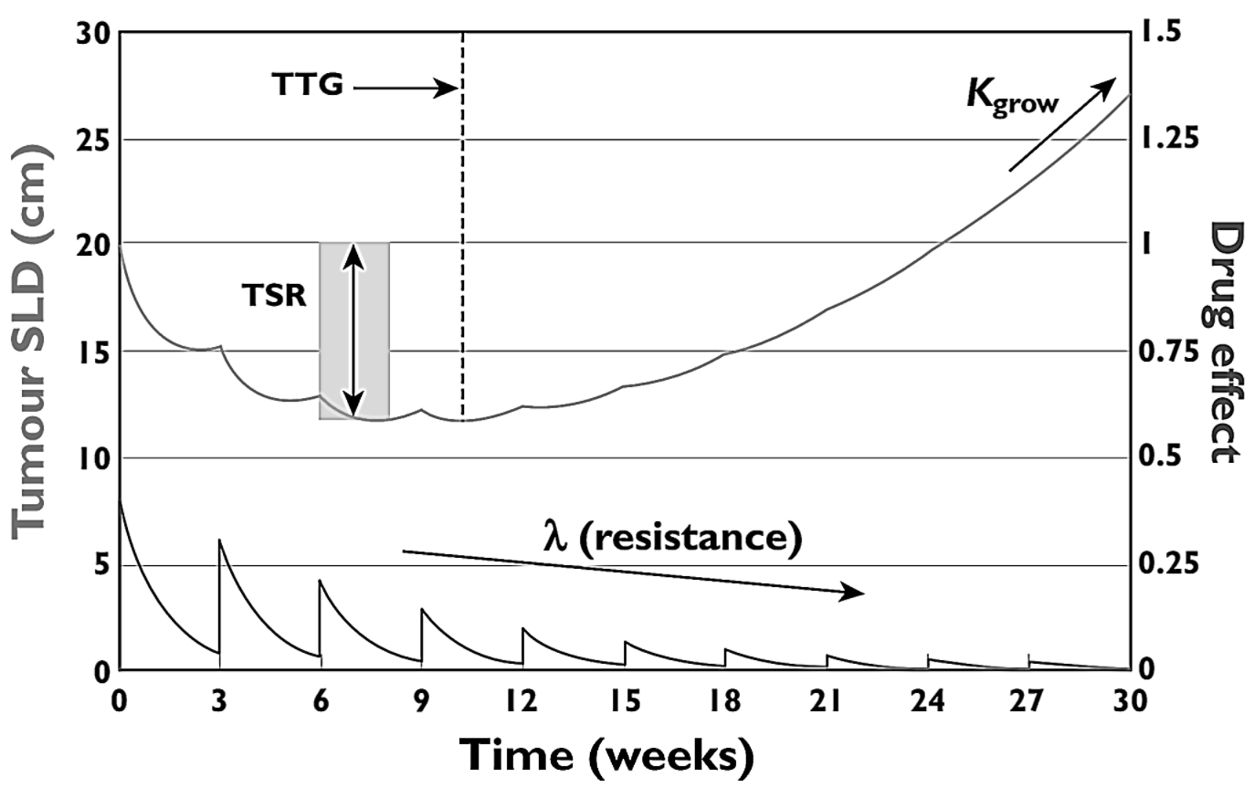
Figure 20 (adapted from Bender, Schindler, and Friberg (2015)) provides an overview of commonly used model-derived tumor growth inhibition (TGI) metrics. The red curve depicts tumor dynamics over time, represented as the sum of longest diameters (SLD), while the blue curve shows the corresponding drug effect. This example uses the Claret et al. (2009) model, where the drug effect diminishes exponentially over time due to the emergence of resistance, governed by the parameter 𝜆. This gradual loss of efficacy leads to eventual tumor regrowth during prolonged treatment. Key TGI metrics illustrated include the tumor shrinkage rate (TSR), time to tumor regrowth (TTG), and the tumor growth rate constant (𝐾grow or kg). These metrics are often used in survival models to characterize treatment response and predict overall survival (OS) or progression free survival (PFS).
Tumor Size Ratio (TSR) The relative change in tumor size from baseline at a fixed time point (e.g., 6–8 weeks):
\(TSR(t) = \frac{TS(t)}{TS_0}\)
Lower TSR values (more shrinkage) are often associated with improved survival.
Time to Tumor Growth (TTG)
Time at which tumor reaches its minimum size before regrowth begins:
\(TTG = \frac{log(K_{kill} \cdot Exposure - log(K_{ge}))}{\lambda}\)
Used in Claret-style models with exponential resistance decay.
Tumor Growth Rate (TGR) or 𝐾g
Reflects how aggressively the tumor grows in the absence of treatment; higher values are typically associated with worse prognosis.
Tumor Size Time-Course [𝑇𝑆(𝑡)]
The full predicted trajectory can be used as a time-varying covariate in survival models (e.g., parametric TTE), preserving more information than static metrics.
Example Use Cases
In colorectal cancer, Claret et al. (2009) demonstrated that model-predicted TSR at week 7 and TTG were significant predictors of OS using parametric survival models.
In renal cell carcinoma, similar metrics were used to extrapolate OS from early tumor kinetics (Stein et al. 2011).
These predictors can be incorporated into parametric time-to-event (TTE) models using metrics like:
\(h(t) = h_0(t) \cdot exp(\beta_1 \cdot TSR + \beta_2 \cdot TTG + ...)\)
5.2 Joint Modeling and Dynamic Predictions
In oncology, it is increasingly valuable to predict long-term outcomes such as overall survival (OS) or progression-free survival (PFS) based on earlier tumor dynamics. This is particularly useful when survival data are immature or delayed, such as in Phase II trials. One effective strategy is joint modeling, where tumor growth inhibition (TGI) and survival processes are modeled together — using model-derived metrics as time-varying or static covariates in a parametric time-to-event (TTE) model.
5.2.1 Survival Submodel (Time-to-Event Component)
A common parametric hazard model used in Pumas is the Weibull model:
\[ h(t) = λ ⋅ γ ⋅ t^{γ−1} ⋅ exp(β_1 ⋅ Z_1 + ⋯ +β_k ⋅ Z_k) \]
Where:
λ, γ: Weibull distribution parameters; baseline hazard shape and scaleZ_k: covariates such as TSR, TTG, or dynamic variable TS(t)β_k: log hazard ratios
Applications of Joint Modeling
Trial simulation: Predict OS curves under new regimens
Bayesian updating: Dynamic prediction of individual risk over time
Early endpoints: Evaluate Go/No-Go decisions based on TSR or TTG
Dose optimization: Link exposure → tumor → survival for MTD or RP2D
6 Summary
Mathematical modeling of tumor dynamics provides a powerful framework to describe, simulate, and predict how tumors grow and respond to anticancer therapies. In this tutorial, we presented a layered, modular approach to tumor growth inhibition (TGI) modeling — starting from basic tumor proliferation functions, progressing through pharmacodynamic drug effects, and culminating in models that capture treatment resistance.
Tumor Growth Models
We introduced a range of tumor growth models — from linear and exponential to more biologically realistic forms such as Gompertz, logistic, power-law, and von Bertalanffy. These models reflect different biological assumptions and are selected based on the tumor type, stage of growth, and data availability.
Drug Effect Models
To model how therapies influence tumor progression, we incorporated drug effect functions ranging from simple direct effects (linear or Emax) to delayed signal-driven models and K-PD approaches used when PK data is absent. These models allow for exploration of dose-response relationships, drug potency, and optimal treatment regimens.
Resistance Models
We also addressed drug resistance, a key driver of tumor relapse. Time-dependent models like the Claret λ model simulate acquired resistance, while fractional resistance models reflect baseline heterogeneity in tumor sensitivity. More mechanistic frameworks like the Proliferative–Quiescent (P–Q) model offer insights into transitions between cellular states and their differential susceptibility to treatment.
Tumor Metrics and Predictive Modeling
TGI models not only simulate longitudinal tumor dynamics, but also provide model-derived metrics that can be used to predict overall survival (OS) or progression-free survival (PFS), such as:
Tumor Size Ratio (TSR): change from baseline at a fixed timepoint,
Time to Tumor Growth (TTG): duration until tumor regrowth begins,
Tumor Growth Rate (TGR): intrinsic aggressiveness of the tumor,
are often incorporated into survival models as covariates. This enables joint modeling strategies where tumor trajectories inform time-to-event predictions — an increasingly valuable tool in oncology development.
Applications
TGI models are used throughout the drug development pipeline:
To simulate tumor response under varying dosing scenarios,
To support first-in-human dose justification and Go/No-Go decisions,
To analyze RECIST-based endpoints (e.g., time to progression),
To explore combination therapies or immuno-oncology mechanisms,
To simulate virtual trials that inform regulatory submissions,
To link early tumor response metrics to survival endpoints using parametric survival models.
7 Additional Reading
For further exploration of tumor growth inhibition modeling, the following references provide comprehensive reviews and applications:
- Ribba et al. (2014) - A review of mixed-effects models of tumor growth and effects of anticancer drug treatment used in population analysis.
- Yin et al. (2019) - A review of mathematical models for tumor dynamics and treatment resistance evolution of solid tumors.
- Bruno et al. (2020) - Progress and opportunities to advance clinical cancer therapeutics using tumor dynamic models.
- Bender, Schindler, and Friberg (2015) - Population pharmacokinetic-pharmacodynamic modelling in oncology: A tool for predicting clinical response.
- Gao et al. (2024) - Realizing the promise of Project Optimus: Challenges and emerging opportunities for dose optimization in oncology drug development.
- Venkatakrishnan and Graaf (2022) - Toward Project Optimus for Oncology Precision Medicine: Multi-Dimensional Dose Optimization Enabled by Quantitative Clinical Pharmacology.
8 References
Belfatto, A, M Riboldi, D Ciardo, A Cecconi, R Lazzari, B A Jereczek-Fossa, R Orecchia, G Baroni, and P Cerveri. 2016. “Adaptive Mathematical Model of Tumor Response to Radiotherapy Based on CBCT Data.” IEEE Journal of Biomedical and Health Informatics 20 (3): 802–9. https://doi.org/10.1109/JBHI.2015.2453437.
Bender, Brendan C, Emilie Schindler, and Lena E Friberg. 2015. “Population Pharmacokinetic-Pharmacodynamic Modelling in Oncology: A Tool for Predicting Clinical Response.” British Journal of Clinical Pharmacology 79 (1): 56–71. https://doi.org/10.1111/bcp.12258.
Bruno, René, Dean Bottino, Dinesh P de Alwis, Antonio T Fojo, Jérémie Guedj, Chao Liu, Kristin R Swanson, Jenny Zheng, Yanan Zheng, and Jin Y Jin. 2020. “Progress and Opportunities to Advance Clinical Cancer Therapeutics Using Tumor Dynamic Models.” Clinical Cancer Research 26 (8): 1787–95. https://doi.org/10.1158/1078-0432.CCR-19-0287.
Bruno, René, Francois Jonsson, Malidi Zaki, Christophe Jacques, Helene Gille, and Bernard Paule. 2012. “Simulations to Assess Phase II Noninferiority Trials of Different Doses of Capecitabine in Combination with Docetaxel for Metastatic Breast Cancer.” CPT: Pharmacometrics & Systems Pharmacology 1: e20. https://doi.org/10.1038/psp.2012.20.
Claret, Laurent, Pascal Girard, Paulo M Hoff, Eric Van Cutsem, Klaas P Zuideveld, Karin Jorga, Jan Fagerberg, and René Bruno. 2009. “Model-Based Prediction of Phase III Overall Survival in Colorectal Cancer on the Basis of Phase II Tumor Dynamics.” Journal of Clinical Oncology 27 (25): 4103–8. https://doi.org/10.1200/JCO.2008.21.0807.
Dansirikul, Chantaratsamon, Helene E Silber, and Mats O Karlsson. 2008. “Approaches to Handling Pharmacodynamic Baseline Responses.” Journal of Pharmacokinetics and Pharmacodynamics 35: 269–83. https://doi.org/10.1007/s10928-008-9088-2.
Eisenhauer, E A, P Therasse, J Bogaerts, L H Schwartz, D Sargent, R Ford, J Dancey, et al. 2009. “New Response Evaluation Criteria in Solid Tumours: Revised RECIST Guideline (Version 1.1).” European Journal of Cancer 45 (2): 228–47. https://doi.org/10.1016/j.ejca.2008.10.026.
Gao, Ying et al. 2024. “Realizing the Promise of Project Optimus: Challenges and Emerging Opportunities for Dose Optimization in Oncology Drug Development.” CPT: Pharmacometrics & Systems Pharmacology. https://doi.org/10.1002/psp4.13079.
Jacqmin, P, E Snoeck, E A van Schaick, R Gieschke, P Pillai, J-L Steimer, and P Girard. 2007. “Modelling Response Time Profiles in the Absence of Drug Concentrations: Definition and Performance Evaluation of the K-PD Model.” Journal of Pharmacokinetics and Pharmacodynamics 34: 57–85. https://doi.org/10.1007/s10928-006-9035-z.
Kühleitner, Manfred, Norbert Brunner, Werner-Georg Nowak, Katharina Renber, and Klara Scheherleitner. 2019. “Best Fitting Tumor Growth Models of the von Bertalanffy-Pütter Type.” BMC Cancer 19: 683. https://doi.org/10.1186/s12885-019-5911-y.
Ollier, Edouard, Pauline Mazzocco, Damien Ricard, Gentian Kaloshi, Ahmed Idbaih, Agusti Alentorn, Dimitri Psimaras, et al. 2017. “Analysis of Temozolomide Resistance in Low-Grade Gliomas Using a Mechanistic Mathematical Model.” Fundamental & Clinical Pharmacology 31 (3): 347–58. https://doi.org/10.1111/fcp.12259.
Ouerdani, A, S Goutagny, M Kalamarides, Iñaki F Trocóniz, and Benjamin Ribba. 2016. “Mechanism-Based Modeling of the Clinical Effects of Bevacizumab and Everolimus on Vestibular Schwannomas of Patients with Neurofibromatosis Type 2.” Cancer Chemotherapy and Pharmacology 77: 1263–73. https://doi.org/10.1007/s00280-016-3046-2.
Ribba, Benjamin, Nick H Holford, Paolo Magni, Iñaki Trocóniz, Ivelina Gueorguieva, Pascal Girard, Christine Sarr, Maya Elishmereni, Charlotte Kloft, and Lena E Friberg. 2014. “A Review of Mixed-Effects Models of Tumor Growth and Effects of Anticancer Drug Treatment Used in Population Analysis.” CPT: Pharmacometrics & Systems Pharmacology 3 (5): e113. https://doi.org/10.1038/psp.2014.12.
Ribba, Benjamin, Gentian Kaloshi, Mathieu Peyre, Damien Ricard, Vincent Calvez, Michel Tod, Branka Çajavec-Bernard, et al. 2012. “A Tumor Growth Inhibition Model for Low-Grade Glioma Treated with Chemotherapy or Radiotherapy.” Clinical Cancer Research 18 (18): 5071–80. https://doi.org/10.1158/1078-0432.CCR-12-0084.
Schindler, Emilie, Michael A Amantea, Mats O Karlsson, and Lena E Friberg. 2017. “A Pharmacometric Framework for Axitinib Exposure, Efficacy, and Safety in Metastatic Renal Cell Carcinoma Patients.” CPT: Pharmacometrics & Systems Pharmacology 6 (6): 373–82. https://doi.org/10.1002/psp4.12193.
Schindler, Emilie, Sreenath M Krishnan, Ron H J Mathijssen, A Ruggiero, G Schiavon, and Lena E Friberg. 2017. “Pharmacometric Modeling of Liver Metastases’ Diameter, Volume, and Density and Their Relation to Clinical Outcome in Imatinib-Treated Patients with Gastrointestinal Stromal Tumors.” CPT: Pharmacometrics & Systems Pharmacology 6 (7): 449–57. https://doi.org/10.1002/psp4.12195.
Stein, Wilfred D, James L Gulley, Jeffrey Schlom, Ravi A Madan, William Dahut, William D Figg, Yiping-M Ning, et al. 2011. “Tumor Regression and Growth Rates Determined in Five Intramural NCI Prostate Cancer Trials: The Growth Rate Constant as an Indicator of Therapeutic Efficacy.” Clinical Cancer Research 17 (4): 907–17. https://doi.org/10.1158/1078-0432.CCR-10-1762.
Stein, Wilfred D, James Yang, Susan E Bates, and Tito Fojo. 2008. “Bevacizumab Reduces the Growth Rate Constants of Renal Carcinomas: A Novel Algorithm Suggests Early Discontinuation of Bevacizumab Resulted in a Lack of Survival Advantage.” The Oncologist 13 (10): 1055–62. https://doi.org/10.1634/theoncologist.2008-0075.
Venkatakrishnan, Karthik, and Piet H van der Graaf. 2022. “Toward Project Optimus for Oncology Precision Medicine: Multi-Dimensional Dose Optimization Enabled by Quantitative Clinical Pharmacology.” Clinical Pharmacology & Therapeutics 112: 927–32. https://doi.org/10.1002/cpt.2742.
Yin, Anyue, Dirk Jan A R Moes, Johan G C van Hasselt, Jesse J Swen, and Henk-Jan Guchelaar. 2019. “A Review of Mathematical Models for Tumor Dynamics and Treatment Resistance Evolution of Solid Tumors.” CPT: Pharmacometrics & Systems Pharmacology 8 (10): 720–37. https://doi.org/10.1002/psp4.12450.