Simulations Strategies from Population Pharmacokinetics Guidance for Industry

Author

Patrick Kofod Mogensen

using Pumas, PharmaDatasets, PumasUtilities, Random, AlgebraOfGraphics, DataFramesMeta
# Set seed
Random.seed!(1234)

TaskLocalRNG()

In this tutorial, we will look at implementing simulations according to Population Pharmacokinetics Guidance for Industry by the US-FDA. The descriptions in the document are non-binding, but they still lay the foundation for a common understanding of what model components should be sampled in different scenarios and which should be held fixed. The document describes three scenarios:

Simulations Based on Fixed-Effect Estimates
Simulations Based on Uncertainty of Fixed-Effects Estimates
Simulations Based on Estimates of Between-Subject Variability

This is all straight forward to do in Pumas and we will show you how to do so in this tutorial.

Some key sources of uncertainty and stochasticity in the pharmacometric models are

Between-subject variability (BSV)
Residual unexplained variability (RUV)

In this context, we could then also add the uncertainty about the exact model specification in terms of the estimated parameters.

1 The Model and Data

We use an existing example data set and model from the PharmaDatasets package.

pk_data = read_pumas(dataset("pumas/sim_data_model1"))

Population
  Subjects: 10
  Observations: dv

We build an model to match the data and call it fda_model

fda_model = @model begin
    @param begin
        θ ∈ VectorDomain(2, init = [0.5, 1.0])
        Ω ∈ PDiagDomain(init = [0.3])
        σ ∈ RealDomain(lower = 0.0, upper = 1.0, init = 0.1)
    end

    @random begin
        η ~ MvNormal(Ω)
    end

    @pre begin
        CL = θ[1] * exp(η[1])
        Vc = θ[2]
    end

    @vars begin
        conc = Central / Vc
    end

    @dynamics Central1

    @derived begin
        dv ~ @. ProportionalNormal(conc, σ)
    end
end

PumasModel
  Parameters: θ, Ω, σ
  Random effects: η
  Covariates:
  Dynamical system variables: Central
  Dynamical system type: Closed form
  Derived: dv, conc
  Observed: dv, conc

The model has a single random effect (whose distribution is represented by a Gaussian distribution with a 1x1 covariance matrix) a single compartment, and a proportional error model.

Using the basic structure of dose events in the population, we re-simulate a new data set at specified time points.

param = init_params(fda_model)
resimulated_data =
    Subject.(
        simobs(
            fda_model,
            pk_data,
            param;
            obstimes = [0.01, 0.5, 1.0, 1.5, 2.0, 2.5, 3.0, 3.5, 4.0],
        )
    )

Population
  Subjects: 10
  Observations: dv

Finally, we fit the model.

ft_dist =
    fit(fda_model, resimulated_data, param, FOCE(); optim_options = (show_trace = false,))
ft_coef = coef(ft_dist)

[ Info: Checking the initial parameter values.
[ Info: The initial negative log likelihood and its gradient are finite. Check passed.

(θ = [0.6086615954498296, 0.9953315556739925], Ω = [0.4374984123998733;;], σ = 0.09098842306105825)

This gives us the primary objects we need:

model: fda_model
dataset: resimulated_data
fit output: ft_dist
estimated fixed effects: ft_coef

When we need parameter uncertainty we will estimate it below.

2 Case I: Simulations Based on Fixed-Effect Estimates

As explained in the guidance, this is the simplest form of simulations. We input the population fixed effects and the center of the random effects. We also plot the trajectories that were simulated. The guidance tells us not to sample observational noise (Residual Unidentified Variability or RUV) here.

eta_center = center_randeffs(fda_model, resimulated_data, ft_coef)
sim_I_1 = simobs(fda_model, resimulated_data, ft_coef, eta_center; simulate_error = false)
sim_plot(sim_I_1)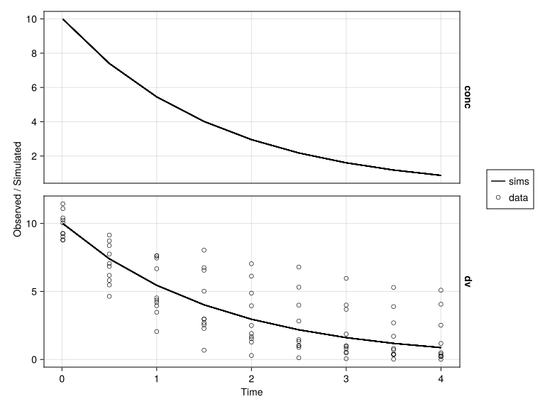

We see that the data used for estimation is spread out, but the simulated trajectories follow the deterministic curve and are all overlapping because there is no heterogeneity coming from covariates.

The default is to simulate with draws from the statistical distribution of the observations. This means that to simulate with observational noise, you don’t need to specify simulate_error, but of course you can manually set it to true as follows:

sim_I_2 = simobs(fda_model, resimulated_data, ft_coef, eta_center; simulate_error = true)
sim_plot(sim_I_2)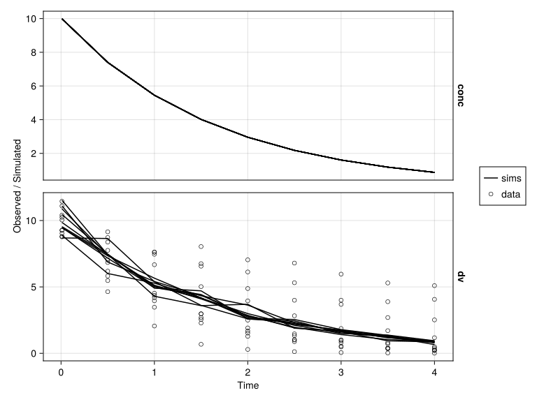

Here we see the same mean tendency, but the blue trajectories are not longer as smooth because there is noise added to the model predictions to match the estimated data generation process. In the guidance, the inclusion of residual error is not mentioned under this section, but is rather delayed to the third section. We will come back to this below.

3 Case II: Simulations Based on Uncertainty of Fixed-Effects Estimates

According to the guidance, simulation with uncertainty of fixed-effects estimates, or very often just “simulation with uncertainty” for short, is for example to be used “if the desire is to illustrate the probability of the typical subject’s drug exposure to reach or stay above a specific cutoff point or if one wishes to illustrate the effect of covariates.” [pp. 13]. They should be used in conjunction with a specific objective in mind and can form the basis of forest plots, effectiveness of new dosing regimens in future trials, or other cases where it’s a good idea to be mindful of the fact that we are not certain about the model parameters and we need some level of precaution when predicting based on the model.

To do these kind of simulations is fairly straight forward. We need some kind of inference first (asymptotic, bootstrap, SIR), and then we can simulate based on that. We use rejection sampling to make sure that parameters stay in their domain as defined in the model.

fda_infer = infer(ft_dist)

[ Info: Calculating: variance-covariance matrix.
[ Info: Done.

Asymptotic inference results using sandwich estimator

Dynamical system type:                 Closed form

Number of subjects:                             10

Observation records:         Active        Missing
    dv:                          90              0
    Total:                       90              0

Number of parameters:      Constant      Optimized
                                  0              4

Likelihood approximation:                     FOCE
Likelihood optimizer:                         BFGS

Termination Reason:              NoObjectiveChange
Log-likelihood value:                   -20.644051

--------------------------------------------------
       Estimate   SE         95.0% C.I.
--------------------------------------------------
θ₁     0.60866    0.12684    [ 0.36007 ; 0.85726]
θ₂     0.99533    0.023598   [ 0.94908 ; 1.0416 ]
Ω₁,₁   0.4375     0.15307    [ 0.13749 ; 0.7375 ]
σ      0.090988   0.00534    [ 0.080522; 0.10145]
--------------------------------------------------

sim_II_1 = simobs(fda_infer, resimulated_data; samples = 80)

sim_II_2 = simobs(fda_infer, resimulated_data, repeat(eta_center, 80); samples = 80)

sim_II_3 = simobs(
    fda_infer,
    resimulated_data,
    repeat(eta_center, 80);
    samples = 80,
    simulate_error = false,
)

This creates a vector of datasets. For each sample of the fixed effects from the uncertainty distribution defined by infer we resimulate resimulated_data and each simulated dataset is an element in the output. In this case, sim_II_3 is then an 80 element vector of SimulatedPopulations.

In some cases such as in forest plots, we may want to simulate a single subject for a number of draws from the uncertainty distribution.

Need More Information?

We encourage you to check out the “A Forest Plot Workflow in Pumas” tutorial to learn more about simulating for forest plots.

4 Case III: Simulations Based on Estimates of Between-Subject Variability

This is the default simulation in Pumas. When you write

simobs(model, population, parameters)

for some model, population, and parameters.

We automatically simulate both between-subject variability (BSV) and residual unexplained variability (RUV). If you wish to be completely transparent about this, it is possible to first sample the random effects and then simulate with RUV added as follows:

eta_sample = sample_randeffs(fda_model, resimulated_data, ft_coef)
sim_III_1 = simobs(fda_model, resimulated_data, ft_coef, eta_sample; simulate_error = true)
sim_plot(sim_III_1)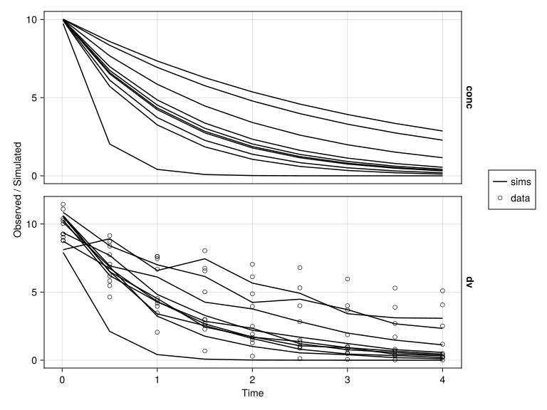

This will essentially do the same as:

sim_III_2 = simobs(fda_model, resimulated_data, ft_coef)
sim_plot(sim_III_1)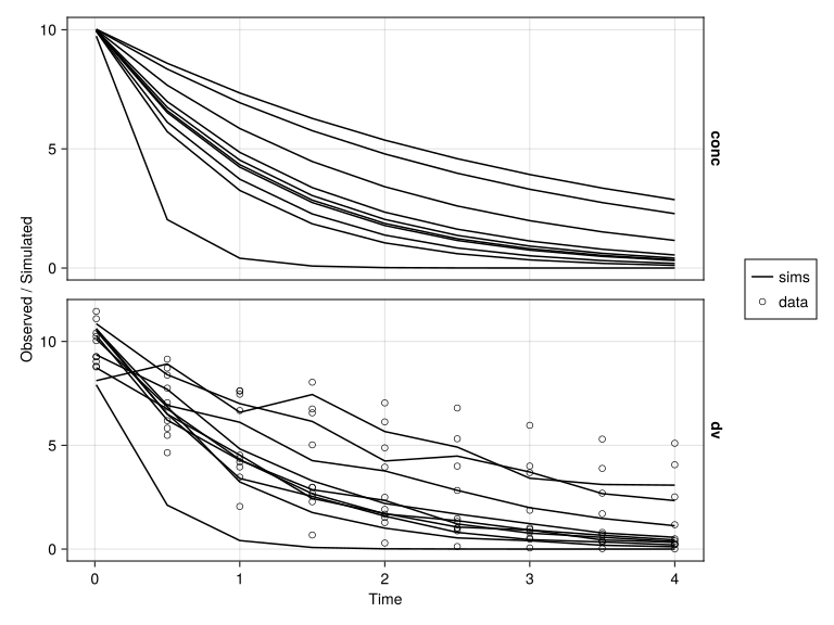

4.1 Comparison of simulations

We can compare the different levels of simulations as follows. First, let us collect all the different versions of the simulation in a DataFrame to compare using AlgebraOfGraphics.

df_I = mapreduce(DataFrame, vcat, sim_II_3)
@rtransform!(df_I, :id = :id * "_II_3")
df_I.Case .= "Uncertainty"
df_III = DataFrame(sim_III_2)
@rtransform!(df_III, :id = :id * "_III_2")
df_III.Case .= "BSV + RUV"
data_df = vcat(df_I, df_III)
@rsubset!(data_df, :evid == 0)

The figure itself can be plotted as boxplots over time with a Case-stratification.

using AlgebraOfGraphics
const AoG = AlgebraOfGraphics
fig = AoG.Figure()
part1 =
    data(data_df) *
    mapping(:time => nonnumeric, :dv, layout = :Case => nonnumeric) *
    visual(AoG.BoxPlot)
draw(part1; legend = (; position = :top))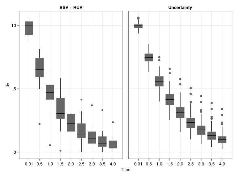

We see that the different simulations have both differences in levels and dispersions due to the different levels of random components sampled and the non-linear nature of the models. This underlines the importance of knowing what type of analysis you wish to perform and how it relates to the recommendations in the Guidance.

5 Conclusion

In this tutorial, we saw how to apply the suggestions of different types of simulations in the Population Pharmacokinetics Guidance for Industry document in Pumas. We saw that there are options to turn the relevant sampling levels on or off and we saw how to generate parameter uncertainty estimates to simulate based on estimated fixed effects and their estimated uncertainty. It is important to remember, that when performing this “simulation with uncertainty” we are also including variability from the random effects themselves.

Reuse

CC BY-SA 4.0