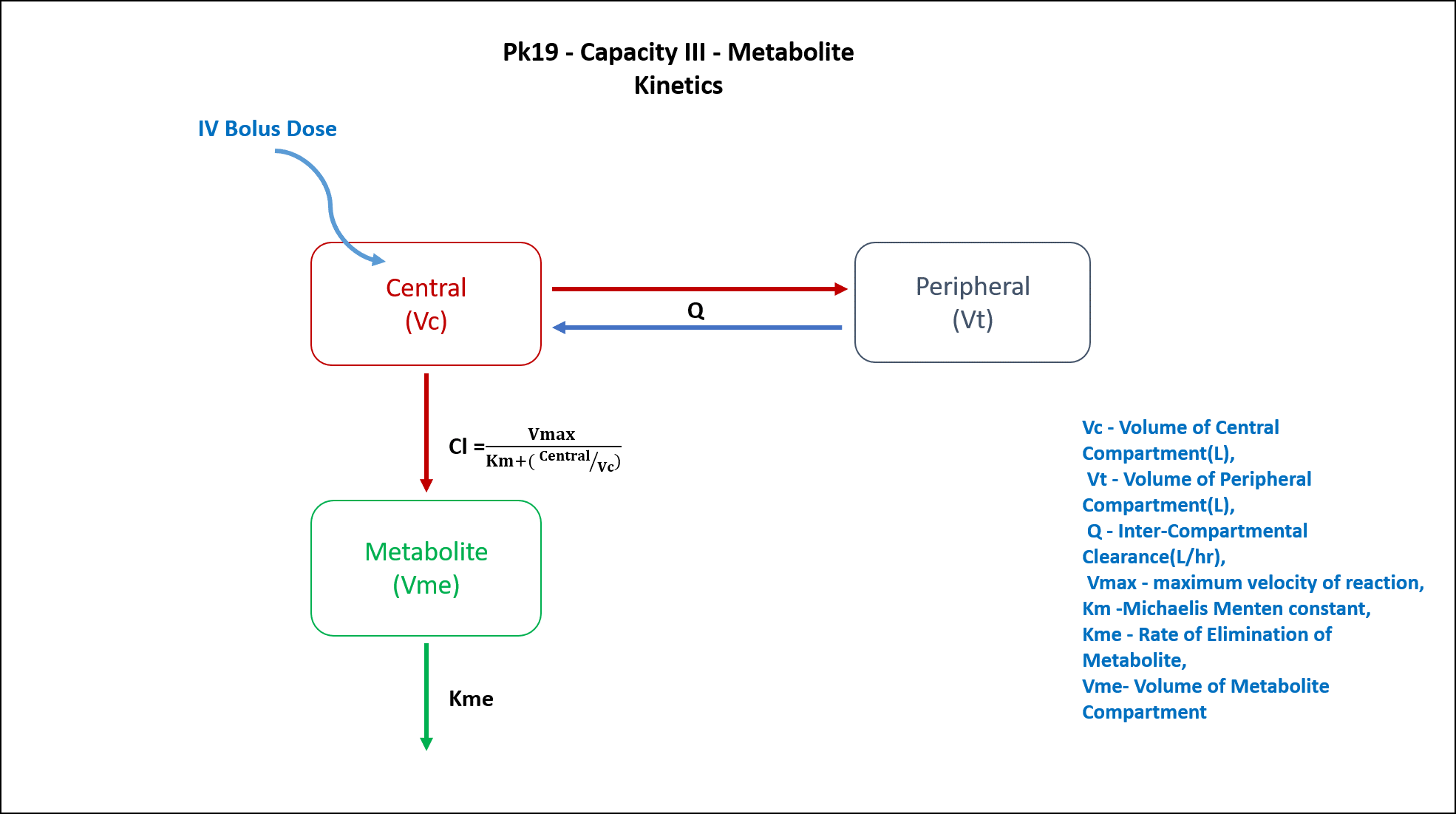
PK19 - Two compartment with limited capacity metabolite model

1 Background

Structural model - Two Compartment model with a Metabolite Compartment
Route of administration - IV Bolus
Dosage Regimen - 10 μmol/kg, 50 μmol/kg, 300 μmol/kg
Number of Subjects - 3

2 Learning Outcome

This exercise demonstrates simulating 3 different doses of a given IV bolus for 3 different subjects.

3 Objectives

To build a two-compartment model, simulate the model for subjects given 3 different IV doses of a drug undergoing capacity limited metabolite kinetics, and subsequently perform simulation for a population.

4 Libraries

Load the necessary libraries.

using PumasUtilities
using Random
using Pumas
using PumasUtilities
using CairoMakie
using AlgebraOfGraphics
using CSV
using DataFramesMeta
using Dates

5 Model definition

Note the expression of the model parameters with helpful comments. The model is expressed with differential equations. Residual variability is a proportional error model.

In this two compartment model, we administer 3 different doses in 3 different subjects of a drug that undergoes metabolite kinetics.

pk_19 = @model begin
    @metadata begin
        desc = "Non-linear formation of Metabolite Model"
        timeu = u"hr"
    end

    @param begin
        """
        Volume of Central Compartment (L/kg)
        """
        tvvc ∈ RealDomain(lower = 0)
        """
        Volume of Perpheral Compartment (L/kg)
        """
        tvvp ∈ RealDomain(lower = 0)
        """
        Inter-Compartmental Clearance (L/min)
        """
        tvq ∈ RealDomain(lower = 0)
        """
        Maximum Velocity of Reaction (μmol/min/kg)
        """
        tvvmax ∈ RealDomain(lower = 0)
        """
        Michaelis-Menten constant (μmol/L)
        """
        tvkm ∈ RealDomain(lower = 0)
        """
        Rate of Elimination of Metabolite (min⁻¹)
        """
        tvkme ∈ RealDomain(lower = 0)
        """
        Volume of Metabolite Compartment (L/kg)
        """
        tvvme ∈ RealDomain(lower = 0)
        #Ω ∈ PDiagDomain(7)
        Ω_vc ∈ RealDomain(lower = 0.0001)
        Ω_vp ∈ RealDomain(lower = 0.0001)
        Ω_q ∈ RealDomain(lower = 0.0001)
        Ω_vmax ∈ RealDomain(lower = 0.0001)
        Ω_km ∈ RealDomain(lower = 0.0001)
        Ω_kme ∈ RealDomain(lower = 0.0001)
        Ω_vme ∈ RealDomain(lower = 0.0001)
        """
        Proportional RUV - Plasma
        """
        σ_prop_cp ∈ RealDomain(lower = 0)
        """
        Proportional RUV - Metabolite
        """
        σ_prop_met ∈ RealDomain(lower = 0)
    end

    @random begin
        η_vc ~ Normal(0, sqrt(Ω_vc))
        η_vp ~ Normal(0, sqrt(Ω_vp))
        η_q ~ Normal(0, sqrt(Ω_q))
        η_vmax ~ Normal(0, sqrt(Ω_vmax))
        η_km ~ Normal(0, sqrt(Ω_km))
        η_kme ~ Normal(0, sqrt(Ω_kme))
        η_vme ~ Normal(0, sqrt(Ω_vme))
    end

    @pre begin
        Vc = tvvc * exp(η_vc)
        Vp = tvvp * exp(η_vp)
        Q = tvq * exp(η_q)
        Vmax = tvvmax * exp(η_vmax)
        Km = tvkm * exp(η_km)
        Kme = tvkme * exp(η_kme)
        Vme = tvvme * exp(η_vme)
    end

    @vars begin
        VMKM := Vmax / (Km + (Central / Vc))
    end

    @dynamics begin
        Central' = -VMKM * (Central / Vc) - (Q / Vc) * Central + (Q / Vp) * Peripheral
        Peripheral' = (Q / Vc) * Central - (Q / Vp) * Peripheral
        Metabolite' = VMKM * (Central / Vc) - Kme * Metabolite
    end

    @derived begin
        cp = @. Central / Vc
        """
        Observed Plasma Concentration (μmol/L)
        """
        dv_cp ~ @. Normal(cp, cp * σ_prop_cp)
        met = @. Metabolite / Vme
        """
        Observed Metabolite Concentration (μmol/L)
        """
        dv_met ~ @. Normal(met, met * σ_prop_met)
    end
end

PumasModel
  Parameters: tvvc, tvvp, tvq, tvvmax, tvkm, tvkme, tvvme, Ω_vc, Ω_vp, Ω_q, Ω_vmax, Ω_km, Ω_kme, Ω_vme, σ_prop_cp, σ_prop_met
  Random effects: η_vc, η_vp, η_q, η_vmax, η_km, η_kme, η_vme
  Covariates: 
  Dynamical system variables: Central, Peripheral, Metabolite
  Dynamical system type: Nonlinear ODE
  Derived: cp, dv_cp, met, dv_met
  Observed: cp, dv_cp, met, dv_met

6 Initial Estimates of Model Parameters

The model parameters for simulation are the following. Note that tv represents the typical value for parameters.

Vc - Volume of Central Compartment (L/kg)
Vp - Volume of Peripheral Compartment (L/kg)
Q - Inter-Compartmental Clearance (L/min)
Vmax - Maximum Velocity of Reaction (μmol/min/kg)
Km - Michaelis-Menten constant (μmol/L)
Kme - Rate of Elimination of Metabolite (min⁻¹)
Vme - Volume of Metabolite Compartment (L/kg)
Ω - Between Subject Variability
σ - Residual error

param = (
    tvvc = 1.06405,
    tvvp = 2.00748,
    tvq = 0.128792,
    tvvmax = 1.64429,
    tvkm = 54.794,
    tvkme = 0.145159,
    tvvme = 0.290811,
    Ω_vc = 0.01,
    Ω_vp = 0.01,
    Ω_q = 0.01,
    Ω_vmax = 0.01,
    Ω_km = 0.01,
    Ω_kme = 0.01,
    Ω_vme = 0.01,
    σ_prop_cp = 0.12,
    σ_prop_met = 0.12,
)

7 Dosage Regimen

Three Subjects were administered three different doses of 10 μmol/kg, 50 μmol/kg and 300 μmol/kg.

dose = [10, 50, 300]

8 Single-individual that receives the defined dose

ids = ["ID:1 Dose 10", "ID:2 Dose 50", "ID:3 Dose 300"]

ev(x) = DosageRegimen(dose[x], cmt = 1, time = 0)

pop = map(zip(1:3, ids)) do (i, id)
    return Subject(id = id, events = ev(i), observations = (cp = nothing, met = nothing))
end

Population
  Subjects: 3
  Observations: cp, met

9 Single-Subject Simulation

Simulate the parent plasma concentration and metabolite plasma concentration.

Initialize the random number generator with a seed for reproducibility of the simulation.

Random.seed!(123)

Define the timepoints at which concentration values will be simulated.

sim_pop3_sub = simobs(pk_19, pop, param, obstimes = 0.1:1:300)

Simulated population (Vector{<:Subject})
  Simulated subjects: 3
  Simulated variables: cp, dv_cp, met, dv_met

9.1 Visualize Results

df_plots = DataFrame(sim_pop3_sub)
first(df_plots, 5)

5×31 DataFrame

Row	id	time	cp	dv_cp	met	dv_met	evid	amt	cmt	rate	duration	ss	ii	route	η_vc_1	η_vp_1	η_q_1	η_vmax_1	η_km_1	η_kme_1	η_vme_1	Central	Peripheral	Metabolite	Vc	Vp	Q	Vmax	Km	Kme	Vme
	String?	Float64	Float64?	Float64?	Float64?	Float64?	Int64?	Float64?	Symbol?	Float64?	Float64?	Int8?	Float64?	NCA.Route?	Float64?	Float64?	Float64?	Float64?	Float64?	Float64?	Float64?	Float64?	Float64?	Float64?	Float64?	Float64?	Float64?	Float64?	Float64?	Float64?	Float64?
1	ID:1 Dose 10	0.0	missing	missing	missing	missing	1	10.0	Central	0.0	0.0	0	0.0	NullRoute	0.107097	-0.0429068	-0.0207674	0.167946	-0.0148676	-0.0958827	-0.0831824	missing	missing	missing	1.18433	1.92317	0.126145	1.94499	53.9854	0.131887	0.267599
2	ID:1 Dose 10	0.1	8.33244	8.42832	0.0970993	0.0851387	0	missing	missing	missing	missing	missing	missing	missing	0.107097	-0.0429068	-0.0207674	0.167946	-0.0148676	-0.0958827	-0.0831824	9.86838	0.105461	0.0259837	1.18433	1.92317	0.126145	1.94499	53.9854	0.131887	0.267599
3	ID:1 Dose 10	1.1	7.32551	9.75397	0.944867	0.785869	0	missing	missing	missing	missing	missing	missing	missing	0.107097	-0.0429068	-0.0207674	0.167946	-0.0148676	-0.0958827	-0.0831824	8.67584	1.05213	0.252846	1.18433	1.92317	0.126145	1.94499	53.9854	0.131887	0.267599
4	ID:1 Dose 10	2.1	6.48584	7.60742	1.5981	1.39125	0	missing	missing	missing	missing	missing	missing	missing	0.107097	-0.0429068	-0.0207674	0.167946	-0.0148676	-0.0958827	-0.0831824	7.68139	1.82638	0.427652	1.18433	1.92317	0.126145	1.94499	53.9854	0.131887	0.267599
5	ID:1 Dose 10	3.1	5.78536	5.69873	2.09364	2.05735	0	missing	missing	missing	missing	missing	missing	missing	0.107097	-0.0429068	-0.0207674	0.167946	-0.0148676	-0.0958827	-0.0831824	6.85179	2.45781	0.560258	1.18433	1.92317	0.126145	1.94499	53.9854	0.131887	0.267599

9.2 Parent

@chain df_plots begin
    dropmissing(:cp)
    data(_) *
    mapping(
        :time => "Time (minutes)",
        :cp => "Parent concentrations (μmol/L)";
        color = :id => "",
    ) *
    visual(Lines; linewidth = 4)
    draw(
        figure = (; fontsize = 22),
        axis = (;
            yscale = log10,
            yticks = map(i -> 10.0^i, -1:2),
            ytickformat = i -> (@. string(round(i; digits = 1))),
            xticks = 0:50:300,
        ),
        legend = (; position = :bottom),
    )
end

9.3 Metabolite

@chain df_plots begin
    dropmissing(:met)
    data(_) *
    mapping(
        :time => "Time (minutes)",
        :met => "Metabolite concentrations (μmol/L)";
        color = :id => "",
    ) *
    visual(Lines; linewidth = 4)
    draw(
        figure = (; fontsize = 22),
        axis = (;
            yscale = log10,
            yticks = map(i -> 10.0^i, -1:2),
            ytickformat = i -> (@. string(round(i; digits = 1))),
            xticks = 0:50:300,
        ),
        legend = (; position = :bottom),
    )
end

10 Population Simulation

We perform a population simulation with 50 participants.

This code demonstrates how to write the simulated concentrations to a comma separated file (.csv).

par = (
    tvvc = 1.06405,
    tvvp = 2.00748,
    tvq = 0.128792,
    tvvmax = 1.64429,
    tvkm = 54.794,
    tvkme = 0.145159,
    tvvme = 0.290811,
    Ω_vc = 0.042,
    Ω_vp = 0.0125,
    Ω_q = 0.0924,
    Ω_vmax = 0.0625,
    Ω_km = 0.0358,
    Ω_kme = 0.0111,
    Ω_vme = 0.0498,
    σ_prop_cp = 0.04587,
    σ_prop_met = 0.0625,
)

ev1 = DosageRegimen(10, cmt = 1, time = 0)
pop1 = map(i -> Subject(id = i, events = ev1), 1:20)
ev2 = DosageRegimen(50, cmt = 1, time = 0)
pop2 = map(i -> Subject(id = i, events = ev2), 21:40)
ev3 = DosageRegimen(300, cmt = 1, time = 0)
pop3 = map(i -> Subject(id = i, events = ev3), 41:60)
pop = [pop1; pop2; pop3]

Random.seed!(1234)
pop_sim = simobs(pk_19, pop, par, obstimes = [0, 5, 10, 20, 30, 60, 90, 120, 180, 300])
sim_plot(pop_sim)

pkdata_19_sim = DataFrame(pop_sim)

#CSV.write("pk_19_sim.csv", pkdata_19_sim);

11 Conclusion

This tutorial showed how to build a two-compartment model with a limited capacity metabolite of a given IV bolus and perform a single subject and population simulation.