using Pumas
using PumasUtilities
using Random
using CairoMakie
using AlgebraOfGraphics
using DataFramesMeta
using CSV
PK38 - Invitro/Invivo extrapolation II
1 Learning Outcome
In this tutorial, we will develop a model to analyze data based on the metabolic rate of a compound using differential equations instead of transforming data into rate versus concentration plot.
2 Background
Before constructing a model, it is important to establish the process the model will follow and a scenario for the simulation.
Below is the scenario for this tutorial:
- Structural Model - Two Enzyme Model
- Route of administration - in vitro experiment
- Dosage regimen - 50, 30, 10, 3, 1 μmol
This diagram describes how such an administered dose will be handled, which facilitates building the model. 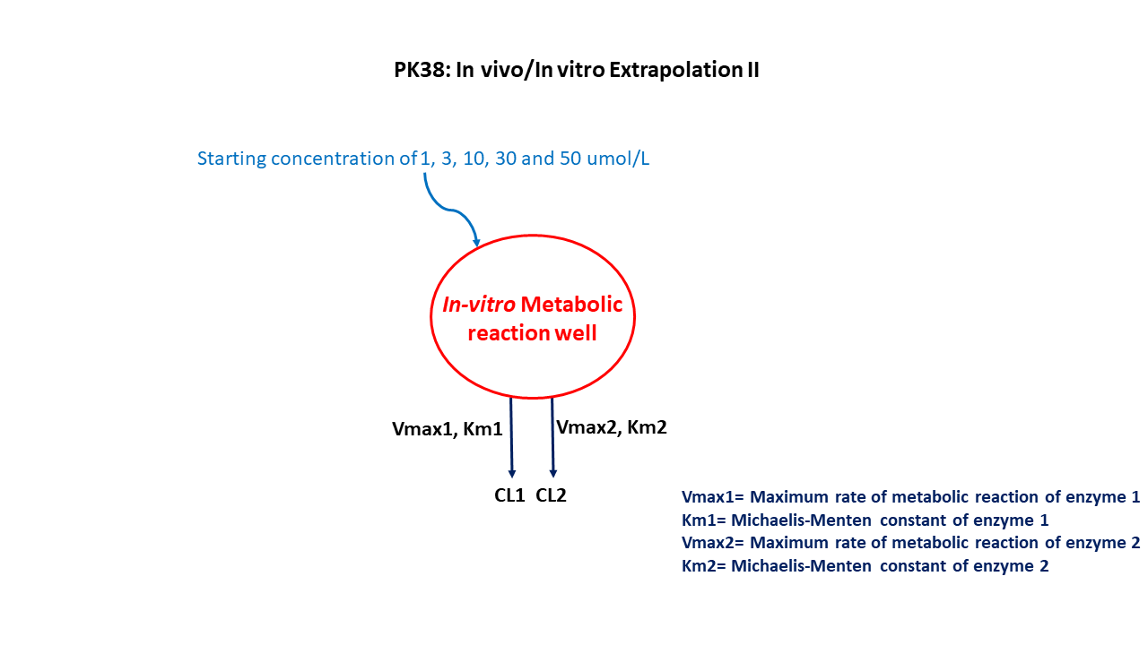
3 Libraries
Call the required libraries to get started.
4 Model
This is a model that depicts the drug passing through two cytochrome P450 isoenzymes (assuming 100% hepatic elimination). Due to this physiologic process, nonlinear elimination for the compound will be applied.
The volume of the incubation medium is set to 1 mL.
pk_38 = @model begin
    @metadata begin
        desc = "Invitro/Invivo Extrapolation Model"
        timeu = u"minute"
    end

    @param begin
        """
        Maximum Metabolic Capacity of System 1 (nmol/min)
        """
        tvvmax1 ∈ RealDomain(lower = 0)
        """
        Michelis Menten Constant of System 1 (μmol/L)
        """
        tvkm1 ∈ RealDomain(lower = 0)
        """
        Maximum Metabolic Capacity of System 2 (nmol/min)
        """
        tvvmax2 ∈ RealDomain(lower = 0)
        """
        Michelis Menten Constant of System 2 (μmol/L)
        """
        tvkm2 ∈ RealDomain(lower = 0)
        Ω ∈ PDiagDomain(4)
        """
        Additive RUV
        """
        σ_add ∈ RealDomain(lower = 0)
    end

    @random begin
        η ~ MvNormal(Ω)
    end

    @pre begin
        Vmax1 = tvvmax1 * exp(η[1])
        Km1 = tvkm1 * exp(η[2])
        Vmax2 = tvvmax2 * exp(η[3])
        Km2 = tvkm2 * exp(η[4])
        Vmedium = 1
    end

    @vars begin
        VMKM := ((Vmax1 * Central / (Km1 + Central)) + (Vmax2 * Central / (Km2 + Central)))
    end

    @dynamics begin
        Central' = -VMKM / Vmedium
    end

    @derived begin
        cp = @. Central / Vmedium
        """
        Observed Concentration (μmol/L)
        """
        dv ~ @. Normal(cp, σ_add)
    end
end
PumasModel
Parameters: tvvmax1, tvkm1, tvvmax2, tvkm2, Ω, σ_add
Random effects: η
Covariates:
Dynamical system variables: Central
Dynamical system type: Nonlinear ODE
Derived: cp, dv
Observed: cp, dv5 Parameters
Parameters provided for simulation are as below.
Vmax1- Maximum Metabolic Capacity of System 1 (nmol/min)Km1- Michelis Menten Constant of System 1 (μmol/l)Vmax2- Maximum Metabolic Capacity of System 2 (nmol/min)Km2- Michelis Menten Constant of System 2 (μmol/l)
These are the initial estimates we will be using in this model exercise. Note that tv represents the typical value for parameters.
param = (;
    tvvmax1 = 0.960225,
    tvkm1 = 0.0896,
    tvvmax2 = 1.01877,
    tvkm2 = 8.67998,
    Ω = Diagonal([0.01, 0.01, 0.01, 0.01]),
    σ_add = 0.02,
)
6 Dosage Regimen
To start the evaluation process, the dosing regimen specified in the background section must be developed first prior to running a simulation.
The dosage regimen is specified as:
Each group is given a different concentration of 50, 30, 10,3 & 5 μmol/L.
This is how to establish one of the dosing regimens:
ev1 = DosageRegimen(50; time = 0, cmt = 1)1×10 DataFrame
| Row | time | cmt | amt | evid | ii | addl | rate | duration | ss | route |
|---|---|---|---|---|---|---|---|---|---|---|
| Float64 | Int64 | Float64 | Int8 | Float64 | Int64 | Float64 | Float64 | Int8 | NCA.Route | |
| 1 | 0.0 | 1 | 50.0 | 1 | 0.0 | 0 | 0.0 | 0.0 | 0 | NullRoute |
This is how to create the single subject undergoing one of the dosing regimen above.
sub1 = Subject(;
    id = "50 μmol/L",
    events = ev1,
    time = [
        0.1,
        0.5,
        1,
        1.5,
        2,
        3,
        4,
        5,
        6,
        7,
        8,
        9,
        10,
        11,
        12,
        13,
        14,
        15,
        16,
        17,
        18,
        19,
        20,
        23,
        27,
        28,
        29,
        30,
        31,
    ],
)
Subject
ID: 50 μmol/L
Events: 1The same previous two steps are repeated for each dosing group below.
ev2 = DosageRegimen(30; time = 0, cmt = 1)1×10 DataFrame
| Row | time | cmt | amt | evid | ii | addl | rate | duration | ss | route |
|---|---|---|---|---|---|---|---|---|---|---|
| Float64 | Int64 | Float64 | Int8 | Float64 | Int64 | Float64 | Float64 | Int8 | NCA.Route | |
| 1 | 0.0 | 1 | 30.0 | 1 | 0.0 | 0 | 0.0 | 0.0 | 0 | NullRoute |
sub2 = Subject(;
    id = "30 μmol/L",
    events = ev2,
    time = [
        0.1,
        0.5,
        1,
        1.5,
        2,
        3,
        4,
        5,
        6,
        7,
        8,
        9,
        10,
        11,
        12,
        13,
        14,
        15,
        16,
        17,
        18,
        19,
        20,
    ],
)
Subject
ID: 30 μmol/L
Events: 1ev3 = DosageRegimen(10; time = 0, cmt = 1)1×10 DataFrame
| Row | time | cmt | amt | evid | ii | addl | rate | duration | ss | route |
|---|---|---|---|---|---|---|---|---|---|---|
| Float64 | Int64 | Float64 | Int8 | Float64 | Int64 | Float64 | Float64 | Int8 | NCA.Route | |
| 1 | 0.0 | 1 | 10.0 | 1 | 0.0 | 0 | 0.0 | 0.0 | 0 | NullRoute |
sub3 = Subject(;
    id = "10 μmol/L",
    events = ev3,
    time = [0.1, 0.5, 1, 1.5, 2, 3, 4, 5, 6, 7, 8],
)
Subject
ID: 10 μmol/L
Events: 1ev4 = DosageRegimen(3; time = 0, cmt = 1)1×10 DataFrame
| Row | time | cmt | amt | evid | ii | addl | rate | duration | ss | route |
|---|---|---|---|---|---|---|---|---|---|---|
| Float64 | Int64 | Float64 | Int8 | Float64 | Int64 | Float64 | Float64 | Int8 | NCA.Route | |
| 1 | 0.0 | 1 | 3.0 | 1 | 0.0 | 0 | 0.0 | 0.0 | 0 | NullRoute |
sub4 = Subject(; id = "3 μmol/L", events = ev4, time = [0.1, 0.5, 1, 1.5, 2, 3])Subject
ID: 3 μmol/L
Events: 1ev5 = DosageRegimen(5; time = 0, cmt = 1)1×10 DataFrame
| Row | time | cmt | amt | evid | ii | addl | rate | duration | ss | route |
|---|---|---|---|---|---|---|---|---|---|---|
| Float64 | Int64 | Float64 | Int8 | Float64 | Int64 | Float64 | Float64 | Int8 | NCA.Route | |
| 1 | 0.0 | 1 | 5.0 | 1 | 0.0 | 0 | 0.0 | 0.0 | 0 | NullRoute |
sub5 = Subject(; id = "5 μmol/L", events = ev5, time = [0.1, 0.5, 1, 1.5])Subject
ID: 5 μmol/L
Events: 1A population is created for each subject with a different dosing regimen.
pop5_sub = [sub1, sub2, sub3, sub4, sub5]Population
Subjects: 5
Observations: 7 Simulation
We will simulate the concentration for the pre-specified time point for each group.
Random.seed!()
The Random.seed! function is included here for purposes of reproducibility of the simulation in this tutorial. Specification of a seed value would not be required in a Pumas workflow that is estimating model parameters.
Random.seed!(123)sim_pop5_sub = simobs(pk_38, pop5_sub, param)Simulated population (Vector{<:Subject})
Simulated subjects: 5
Simulated variables: cp, dvThis line demonstrates how to see the simulation results in a DataFrame and will be important for the following visualization step.
df38 = DataFrame(sim_pop5_sub)
first(df38, 3)
3×22 DataFrame
| Row | id | time | cp | dv | evid | amt | cmt | rate | duration | ss | ii | route | η_1 | η_2 | η_3 | η_4 | Central | Vmax1 | Km1 | Vmax2 | Km2 | Vmedium |
|---|---|---|---|---|---|---|---|---|---|---|---|---|---|---|---|---|---|---|---|---|---|---|
| String? | Float64 | Float64? | Float64? | Int64? | Float64? | Symbol? | Float64? | Float64? | Int8? | Float64? | NCA.Route? | Float64? | Float64? | Float64? | Float64? | Float64? | Float64? | Float64? | Float64? | Float64? | Int64? | |
| 1 | 50 μmol/L | 0.0 | missing | missing | 1 | 50.0 | Central | 0.0 | 0.0 | 0 | 0.0 | NullRoute | 0.0516143 | 0.0091941 | -0.172806 | 0.109577 | missing | 1.01109 | 0.0904276 | 0.857092 | 9.68517 | 1 |
| 2 | 50 μmol/L | 0.1 | 49.8273 | 49.8338 | 0 | missing | missing | missing | missing | missing | missing | missing | 0.0516143 | 0.0091941 | -0.172806 | 0.109577 | 49.8273 | 1.01109 | 0.0904276 | 0.857092 | 9.68517 | 1 |
| 3 | 50 μmol/L | 0.5 | 49.1369 | 49.1444 | 0 | missing | missing | missing | missing | missing | missing | missing | 0.0516143 | 0.0091941 | -0.172806 | 0.109577 | 49.1369 | 1.01109 | 0.0904276 | 0.857092 | 9.68517 | 1 |
8 Visualization
This step wrangles the data to create the plot. This step may look different from other plots in other tutorials, but really is two steps from the same process merged into one step.
With dropmissing(), we are eliminating any missing values (in this case, this will be missing values in :cp, plasma concentration). Next is the setup for the AlgebraOfGraphics plot creation with the common structure denoted below:
dose_sorter = sorter("3 μmol/L", "5 μmol/L", "10 μmol/L", "30 μmol/L", "50 μmol/L")
@chain df38 begin
    dropmissing(:cp)
    data(_) *
    mapping(
        :time => "Time (min)",
        :cp => "Concentration (μmol/L)",
        color = :id => dose_sorter => "Dose",
    ) *
    visual(ScatterLines, linewidth = 4, markersize = 12)
    draw(;
        figure = (; fontsize = 22),
        axis = (;
            xticks = 0:5:35,
            yscale = Makie.pseudolog10,
            ytickformat = i -> (@. string(round(i; digits = 1))),
        ),
    )
end
9 Population Simulation
This block updates the parameters of the model to increase intersubject variability in parameters and defines timepoints for prediction of concentrations. The results are written to a CSV file.
par = (
    tvvmax1 = 0.960225,
    tvkm1 = 0.0896,
    tvvmax2 = 1.01877,
    tvkm2 = 8.67998,
    Ω = Diagonal([0.012, 0.021, 0.018, 0.032]),
    σ_add = 0.04,
)

ev1 = DosageRegimen(50; time = 0, cmt = 1)
pop1 = map(
    i -> Subject(
        id = i,
        events = ev1,
        covariates = (Group = "1",),
        time = [
            0.1,
            0.5,
            1,
            1.5,
            2,
            3,
            4,
            5,
            6,
            7,
            8,
            9,
            10,
            11,
            12,
            13,
            14,
            15,
            16,
            17,
            18,
            19,
            20,
            23,
            27,
            28,
            29,
            30,
            31,
        ],
    ),
    1:6,
)
ev2 = DosageRegimen(30; time = 0, cmt = 1)
pop2 = map(
    i -> Subject(
        id = i,
        events = ev2,
        covariates = (Group = "2",),
        time = [
            0.1,
            0.5,
            1,
            1.5,
            2,
            3,
            4,
            5,
            6,
            7,
            8,
            9,
            10,
            11,
            12,
            13,
            14,
            15,
            16,
            17,
            18,
            19,
            20,
        ],
    ),
    7:12,
)
ev3 = DosageRegimen(10; time = 0, cmt = 1)
pop3 = map(
    i -> Subject(
        id = i,
        events = ev3,
        covariates = (Group = "3",),
        time = [0.1, 0.5, 1, 1.5, 2, 3, 4, 5, 6, 7, 8],
    ),
    13:18,
)
ev4 = DosageRegimen(3; time = 0, cmt = 1)
pop4 = map(
    i -> Subject(
        id = i,
        events = ev4,
        covariates = (Group = "4",),
        time = [0.1, 0.5, 1, 1.5, 2, 3],
    ),
    19:24,
)
ev5 = DosageRegimen(1; time = 0, cmt = 1)
pop5 = map(
    i -> Subject(
        id = i,
        events = ev5,
        covariates = (Group = "5",),
        time = [0.1, 0.5, 1, 1.5],
    ),
    25:30,
)
These are the overall results:
pop = [pop1; pop2; pop3; pop4; pop5]

Random.seed!(1234)
sim_pop = simobs(pk_38, pop, par)

df_sim = DataFrame(sim_pop)

#CSV.write("pk_38.csv", df_sim)
Saving the Simulation Results
With the CSV.write function, you can input the name of the dataframe (df_sim) and the file name of your choice (pk_38.csv) to save the file to your local directory or repository.
10 Conclusion
Constructing a model based on the metabolic rate of a compound involves:
- understanding the process of how the drug is passed through the system,
- translating processes into differential equations using Pumas, and
- simulating the model in a single patient for evaluation.