using Dates
using Pumas
using PumasUtilities
using CairoMakie
using DataFramesMeta
using PharmaDatasets
Fitting models with Pumas
Caution
Some functions in this tutorial are only available after you load the PumasUtilities package.
In this tutorial we will go through the steps required to fit a model in Pumas.
We’ll show two models:
- proportional error model
- additive error model
Additionally, we’ll learn how to compare both models and make a decision on which model is more appropriate for the data.
1 Pumas’ workflow
- Define a model. It can be a
PumasModelor aPumasEMModel. - Define a
SubjectandPopulation. - Fit your model.
- Perform inference on the model’s population-level parameters (also known as fixed effects).
- Predict from a fitted model using the empirical Bayes estimate or Simulate random observations from a fitted model using the sampling distribution (also known as likelihood).
- Model diagnostics and visual predictive checks.
Note
Pumas modeling is a highly iterative process. Eventually you’ll probably go back and forth in the stages of workflow. This is natural and expected in Pumas’ modeling. Just remember to have good code organization and version control for all of the workflow iterations.
Tip
Objects of PumasModel are created with the @model macro and they represent NLME models, i.e. models that we fit with iterative maximum likelihood estimates with first order (conditional) dynamics FO/FOCE/LaplaceI.
PumasEMModel are created with the @emmodel macro and they represent SAEM models, i.e. models that we fit using stochastic aproximation of the expectation-maximization estimation method.
1.1 Defining a model in Pumas
To define a model in Pumas, you can use either the macros or the function interfaces. We will cover the macros interface in this lesson.
To define a model using the macro interface, you start with a begin .. end block of code with @model:
my_model = @model begin endPumasModel
Parameters:
Random effects:
Covariates:
Dynamical system variables:
Dynamical system type: No dynamical model
Derived:
Observed:This creates an empty model. Now we need to populate it with model components. These are additional macros that we can include inside the @model definition. We won’t be covering all the possible macros that we can use in this lesson, but here is the full list:
@param, fixed effects specifications.@random, random effects specifications.@covariates, covariate names.@pre, pre-processing variables for the dynamic system and statistical specification.@dosecontrol, specification of any dose control parameters present in the model.@vars, shorthand notation.@init, initial conditions for the dynamic system.@dynamics, dynamics of the model.@derived, statistical modeling of dependent variables.@observed, model information to be stored in the model solution.
Note
The model components are marked by special macros. A macro in Julia behaves somewhat like a function and is marked with a @ character. These model components should be placed inside the @model macro.
1.1.1 Model parameters with @param
Ok, let’s start with our model_proportional using the macro @model interface.
First, we’ll define our parameters with the @param macro:
@param begin
    ParameterName ∈ Domain(...)
    ...
end
Tip
To use the “in” (∈) operator in Julia, you can either replace ∈ for in or type \in <TAB> for the Unicode character.
By using the begin ... end block we can specify one parameter per line.
Regarding the Domain(...), Pumas has several types of domains for you to specify in your @param block. Here is a list:
RealDomainfor scalar parametersVectorDomainfor vectorsPDiagDomainfor positive definite matrices with diagonal structurePSDDomainfor general positive semi-definite matrices
Tip
PDiagDomain and PSDDomain are generally used for between-subject variability (BSV) covariance matrices.
By using PDiagDomain we are implying that the BSV are independent, i.e. they are not allowed to have covariance, since the off-diagonal elements are turned off by default.
Whereas, by using PSDDomain we are implying that the BSV are not independent, i.e. they are allowed to have covariance, since we have a full covariance matrix instead of a diagonal one.
Tip
If you don’t specify any arguments inside the domain constructor it will either error (for some domains that have required arguments) or will use the defaults. In the case of the RealDomain() without arguments it just uses the following arguments:
RealDomain(; lower = -∞, upper = ∞, init = 0)@param begin
tvcl ∈ RealDomain(; lower = 0) # typical clearance
tvvc ∈ RealDomain(; lower = 0) # typical central volume of distribution
Ω ∈ PDiagDomain(2) # between-subject variability
σ ∈ RealDomain(; lower = 0) # residual variability
end
Note
We will be using the convention to name population-specific parameters (also commonly referred to as typical values) as tv*.
For example, typical clearance will be named as tvcl.
1.1.2 Subject parameters with @random
Second, we’ll define our subject-specific parameters (commonly known as our etas, η, or random effects) with the @random macro:
@random begin
    η ~ MvNormal(Ω) # multi-variate Normal with mean 0 and covariance matrix Ω
end
Here we are using the random assignment with the tilde notation, as in η ~ Distribution(...). This means that the parameter η is distributed as some distribution Distribution with certain parameters.
In our case, η comes from a multivariate normal distribution (MvNormal) with a single positional argument Ω which itself is a positive diagonal covariance matrix. This way of instantiating a multivariate normal distribution implies that the mean vector is a vector filled with 0s. Hence, our η is a vector of the same length as Ω’s dimensionality, i.e. vector of length 2.
Tip
You can use any distribution in the @random block. For a full list of distributions, check the Pumas @random documentation.
You don’t need to be constrained to normal or multivariate normal. Don’t forget to check the Beyond Gaussian Random Effects tutorial.
1.1.3 Pre-processing variables with @pre
We can specify all the necessary variable and statistical pre-processing with the @pre macro.
Note
The @pre block is traditionally used to specify the inputs of the Ordinary Differential Equations (ODE) system used for non-linear mixed-effects PK/PD models (NLME).
We can also use @pre to specify variable transformations.
Here, we are defining all the individual PK parameters, i.e. the typical values with the added ηs:
@pre begin
    CL = tvcl * exp(η[1])
    Vc = tvvc * exp(η[2])
end
Note
We will be using the convention to name subject-specific PK parameters (also commonly referred to as individual coefficients or icoefs) with uppercase.
For example, the subject-specific clearance parameter will be named as CL.
1.1.4 Model dynamics with @dynamics
The next block is the @dynamics blocks. Here we specify all of the model’s dynamics, i.e. the ordinary differential equation (ODE) system:
@dynamics begin
    Central' = -CL / Vc * Central
end
We specify one ODE per line inside the @dynamics block. The syntax is:
Compartment' = transformation * CompartmentThis means that the rate of change, i.e. the derivative, of the compartment Compartment is equal to a transformation of the current values of the compartment Compartment. It is very similar to the textbook/paper math notation that you see in most pharmacometrics resources.
We can name our compartments whatever we want. In our example, we are naming the central compartment simply as Central.
Tip
You can also use aliases for the most common compartment models as a shortcut. Check the Pumas documentation on the predefined ODEs.
For example, the Central1 alias corresponds to the following @dynamics block:
Central' = -(CL / Vc) * CentralIf you are using the aliases, don’t forget to adjust the variables’ naming in the @pre block accordingly.
Note
Under the hood Pumas performs some checks on your ODE system specified in the @dynamics block.
First, Pumas will check if the ODE is linear, and, if possible, will replace your ODE system by a simple matrix exponentiation operation, which is faster than the analytical closed form solution.
Second, Pumas will check if the ODE system is a stiff ODE system, and adjust the numerical solver accordingly.
This means that you don’t need to think about numerical details of your ODE system. Just focus on the dynamics and let Pumas take care of the rest.
1.1.5 Statistical modeling of dependent variables with @derived
Our final block, @derived, is used to specify all the assumed distributions of observed variables that are derived from the blocks above. This is where we include our dependent variable/observation: dv and any other intermediate values that we need to calculate:
@derived begin
    cp := @. 1_000 * Central / Vc # Change of units
    dv ~ @. ProportionalNormal(cp, σ)
end
Note that dv is being declared as following a ProportionalNormal distribution with the same tilde notation ~ as we used in the @random block. It means (much like the mathematical model notation) that dv follows a proportional normal distribution, i.e., a normal distribution whose standard deviation is proportional to its mean. Since dv is a vector of values, we need to broadcast, i.e. vectorize, the operation with the dot . operator:
dv ~ Normal.(μ, σ)where μ and σ are the parameters that parametrizes the distribution, and in this case are the mean and standard deviation respectively. We can use the @. macro which tells Julia to apply the . in every operator and function call after it:
dv ~ @. Normal(μ, σ)
Note
We are using the @. macro which tells Julia to vectorize (add the “dot syntax”) to all operations and function calls to the right of it.
Additionally, we are also calculating an intermediate variable cp which represents the concentration in plasma.
Here we are using the := assignment, which marks cp as a deterministic intermediate quantity that is only used inside the @derived block. Its value is the Central compartment divided by the individual volume of the Central compartment PK parameter, Vc, scaled by a thousands units. Hence, the multiplication by a 1_000. If we also wanted cp to be returned when simulating from the model, we would define it in a separate @observed block instead.
Tip
In this block we can use all variables defined in the previous blocks, in our example the @param, @dynamics and @pre blocks.
1.1.6 Creating two different Pumas models
We now proceed by creating two different Pumas models. Both of them are 1-compartment IV models, but with different error models.
Note
The additive error model has a parameter σ inside the @derived block that, contrary to the proportional error model, is not multiplied by the mean cp:
dv ~ @. Normal(cp, σ)model_proportional = @model begin
@param begin
# here we define the parameters of the model
tvcl ∈ RealDomain(; lower = 0) # typical clearance
tvvc ∈ RealDomain(; lower = 0) # typical central volume of distribution
Ω ∈ PDiagDomain(2) # between-subject variability
σ ∈ RealDomain(; lower = 0) # residual variability
end
@random begin
# here we define random effects
η ~ MvNormal(Ω) # multi-variate Normal with mean 0 and covariance matrix Ω
end
@pre begin
# pre computations and other statistical transformations
CL = tvcl * exp(η[1])
Vc = tvvc * exp(η[2])
end
# here we define compartments and dynamics
@dynamics begin
Central' = -CL / Vc * Central
end
@derived begin
# here is where we calculate concentration and add residual error
# tilde (~) means "distributed as"
cp := @. 1_000 * Central / Vc # Change of units
dv ~ @. ProportionalNormal(cp, σ)
end
endPumasModel
Parameters: tvcl, tvvc, Ω, σ
Random effects: η
Covariates:
Dynamical system variables: Central
Dynamical system type: Matrix exponential
Derived: dv
Observed: dvmodel_additive = @model begin
@param begin
# here we define the parameters of the model
tvcl ∈ RealDomain(; lower = 0) # typical clearance
tvvc ∈ RealDomain(; lower = 0) # typical central volume of distribution
Ω ∈ PDiagDomain(2) # between-subject variability
σ ∈ RealDomain(; lower = 0) # residual variability
end
@random begin
# here we define random effects
η ~ MvNormal(Ω) # multi-variate Normal with mean 0 and covariance matrix Ω
end
@pre begin
# pre computations and other statistical transformations
CL = tvcl * exp(η[1])
Vc = tvvc * exp(η[2])
end
# here we define compartments and dynamics
@dynamics begin
Central' = -CL / Vc * Central
end
@derived begin
# here is where we calculate concentration and add residual error
# tilde (~) means "distributed as"
cp := @. 1_000 * Central / Vc # Change of units
dv ~ @. Normal(cp, σ)
end
endPumasModel
Parameters: tvcl, tvvc, Ω, σ
Random effects: η
Covariates:
Dynamical system variables: Central
Dynamical system type: Matrix exponential
Derived: dv
Observed: dv1.2 Define a Subject and Population
Once we have our model defined we have to specify a Subject or a Population.
In Pumas, subjects are represented by the Subject type and collections of subjects are represented as vectors of Subjects are defined as Population.
Subjects can be constructed with the Subject constructor, for example:
Subject(; id = 1)Subject
ID: 1We just constructed a Subject that has ID equal to 1 and no extra information.
Since a Population is just a vector of Subjects, we can use a simple map function over the a list of IDs:
pop1 = map(i -> Subject(; id = i), 1:10)Population
Subjects: 10
Observations: Or we can construct the vector of Subjects manually:
pop2 = [Subject(; id = 1), Subject(; id = 2)]Population
Subjects: 2
Observations: pop1 isa Populationtruepop2 isa PopulationtrueAs you can see a Vector of Subjects will always be a Population.
1.2.1 Reading Subjects directly from a DataFrame
Of course we don’t want to create Subjects and Populations manually. We generally have the data represented in some sort of tabular data format, e.g. CSV or Excel files.
Tip
Don’t forget to check the Data Wrangling - Reading and Writing Data tutorial.
We can parse a DataFrame into a Population (or Subject in the case of a single subject data) with the read_pumas function.
The read_pumas function accepts as first argument a DataFrame followed by the following keyword arguments:
observations: dependent variables specified by a vector of column names, i.e.[:DV].covariates: covariates specified by a vector of column names.id: specifies the unique Subject ID column of theDataFrame.time: specifies the time column of theDataFrame.amt: specifies the amount column of theDataFrame.evid: specifies the event unique ID (EVID) column of theDataFrame.
Tip
The read_pumas function has more keywords arguments and options than described above. Don’t forget to check the Pumas documentation on read_pumas.
1.2.2 The iv_sd_3 dataset
In our example, we’ll be using the iv_sd_3 (intravenous single dose 3) dataset from the PharmaDatasets package. This package has several pharma-related datasets ready to be used in the most common pharmacometrics workflows, such as in our example, PK model fitting.
pkdata = dataset("iv_sd_3")
first(pkdata, 5)
5×9 DataFrame
| Row | id | time | cp | dv | amt | evid | cmt | rate | dosegrp |
|---|---|---|---|---|---|---|---|---|---|
| Int64 | Float64 | Float64? | Float64? | Float64? | Int64 | Int64 | Float64 | Int64 | |
| 1 | 1 | 0.0 | missing | missing | 10.0 | 1 | 1 | 0.0 | 10 |
| 2 | 1 | 0.25 | 239.642 | 233.091 | missing | 0 | 1 | 0.0 | 10 |
| 3 | 1 | 0.5 | 235.243 | 270.886 | missing | 0 | 1 | 0.0 | 10 |
| 4 | 1 | 0.75 | 230.925 | 309.181 | missing | 0 | 1 | 0.0 | 10 |
| 5 | 1 | 1.0 | 226.687 | 269.433 | missing | 0 | 1 | 0.0 | 10 |
Let’s see how many different EVIDs rows we have per subject:
@by pkdata :id begin
    :EVID_0 = count(==(0), :evid)
    :EVID_1 = count(==(1), :evid)
end
last(pkdata, 5)
5×9 DataFrame
| Row | id | time | cp | dv | amt | evid | cmt | rate | dosegrp |
|---|---|---|---|---|---|---|---|---|---|
| Int64 | Float64 | Float64? | Float64? | Float64? | Int64 | Int64 | Float64 | Int64 | |
| 1 | 120 | 24.0 | 366.994 | 449.561 | missing | 0 | 1 | 0.0 | 120 |
| 2 | 120 | 36.0 | 147.526 | 129.685 | missing | 0 | 1 | 0.0 | 120 |
| 3 | 120 | 48.0 | 59.3031 | 67.6517 | missing | 0 | 1 | 0.0 | 120 |
| 4 | 120 | 60.0 | 23.8389 | 22.5353 | missing | 0 | 1 | 0.0 | 120 |
| 5 | 120 | 71.9 | 9.65593 | 14.4299 | missing | 0 | 1 | 0.0 | 120 |
Tip
We won’t be covering data wrangling here. Please check the Pumas Data Wrangling tutorials.
As you can see, we have 120 subjects each with one dosing row (evid == 1)and 15 measurement rows (evid == 0).
Each one of the subjets is being given a dose of 10 units intravenous at time 0.
Additionally we have a :dv column with the observations for the measurement rows.
Let’s parse the pkdata DataFrame into a Population with the read_pumas function:
pop = read_pumas(
    pkdata;
    observations = [:dv],
    id = :id,
    time = :time,
    amt = :amt,
    evid = :evid,
)
Population
Subjects: 120
Observations: dv1.3 Fit your model
Now we are ready to fit our model! We already have a model specified, model_proportional and model_additive, along with a Population: pop. We can proceed with model fitting.
Model fiting in Pumas has the purpose of estimating parameters and is done by calling the fit function with the following positional arguments:
- Pumas model.
- a
Population. - a named tuple of the initial parameter values.
- an inference algorithm.
1.3.1 Initial Parameter Values
We already covered model and Population, now let’s talk about initial parameter values. It is the 3rd positional argument inside fit.
You can specify you initial parameters as a named tuple. For instance, if you want to have a certain parameter, tvcl, as having an initial value as 1, you can do so by passing it inside a named tuple in the 3rd positional argument of fit:
fit(model, population, (; tvcl = 1.0))
Tip
You can also use the helper function init_params which will recover all the initial parameters we specified inside the model’s @param block.
Let’s define a named tuple with the initial parameters values and name it iparams:
iparams = (; tvcl = 1, tvvc = 10, Ω = Diagonal([0.09, 0.09]), σ = 0.3)(tvcl = 1, tvvc = 10, Ω = [0.09 0.0; 0.0 0.09], σ = 0.3)
Note
For Ω, since it lies in the PDiagDomain, we are using a diagonal matrix (created with Diagonal by passing a vector where the components are the diagonal entries) as the initial value.
1.3.2 Inference Algorithms
Finally, our last (4th) positional argument is the choice of inference algorithm.
Pumas has the following available inference algorithms:
Marginal Likelihood Estimation:
NaivePooled(): first order approximation without random-effects.FO(): first-order approximation.FOCE(): first-order conditional estimation with automatic interaction detection.LaplaceI(): second-order Laplace approximation.
Bayesian with Markov Chain Monte Carlo (MCMC):
BayesMCMC(): MCMC using No-U-Turn Sampler (NUTS).
Note
We can also use a Maximum A Posteriori (MAP) estimation procedure for any marginal likelihood estimation algorithm. You just need to call the MAP() constructor with the desired marginal likelihood algorithm inside, for instance:
fit(model, population, init_params(model), MAP(FOCE()))Ok, we are ready to fit our model. Let’s use the FOCE:
fit_proportional = fit(model_proportional, pop, iparams, FOCE())[ Info: Checking the initial parameter values. [ Info: The initial negative log likelihood and its gradient are finite. Check passed. Iter Function value Gradient norm 0 1.287102e+04 2.175890e+03 * time: 0.03348803520202637 1 9.966790e+03 7.267813e+02 * time: 3.7215840816497803 2 9.530310e+03 5.388719e+02 * time: 3.7942070960998535 3 9.441794e+03 1.704334e+02 * time: 3.8609869480133057 4 9.413161e+03 7.105680e+01 * time: 3.9289891719818115 5 9.408707e+03 4.180099e+01 * time: 4.003184080123901 6 9.404627e+03 3.771692e+01 * time: 4.078772068023682 7 9.402418e+03 3.621230e+01 * time: 4.151832103729248 8 9.400119e+03 3.839299e+01 * time: 4.221415996551514 9 9.396350e+03 7.333659e+01 * time: 4.286599159240723 10 9.389051e+03 1.097953e+02 * time: 4.351534128189087 11 9.379940e+03 9.319034e+01 * time: 4.488917112350464 12 9.376311e+03 2.014382e+01 * time: 4.552894115447998 13 9.375988e+03 1.192272e+01 * time: 4.615648984909058 14 9.375925e+03 4.549414e+00 * time: 4.68088698387146 15 9.375900e+03 4.852128e+00 * time: 4.742759943008423 16 9.375861e+03 4.819367e+00 * time: 4.809389114379883 17 9.375777e+03 4.366775e+00 * time: 4.8775341510772705 18 9.375687e+03 4.860785e+00 * time: 4.947193145751953 19 9.375637e+03 2.345193e+00 * time: 5.060556173324585 20 9.375629e+03 4.676145e-01 * time: 5.11978816986084 21 9.375628e+03 2.889475e-02 * time: 5.1785149574279785 22 9.375628e+03 1.919844e-03 * time: 5.234131097793579 23 9.375628e+03 1.919662e-03 * time: 5.332486152648926 24 9.375628e+03 1.919662e-03 * time: 5.481783151626587
FittedPumasModel

Dynamical system type:          Matrix exponential

Number of subjects:                            120

Observation records:         Active        Missing
    dv:                        1799              0
    Total:                     1799              0

Number of parameters:      Constant      Optimized
                                  0              5

Likelihood approximation:                     FOCE
Likelihood optimizer:                         BFGS

Termination Reason:                      NoXChange
Log-likelihood value:                   -9375.6282

-----------------
       Estimate
-----------------
tvcl    3.8588
tvvc   70.902
Ω₁,₁    0.092946
Ω₂,₂    0.086108
σ       0.20577
-----------------
fit_additive = fit(model_additive, pop, iparams, FOCE())[ Info: Checking the initial parameter values. [ Info: The initial negative log likelihood and its gradient are finite. Check passed. Iter Function value Gradient norm 0 1.588465e+08 3.176814e+08 * time: 1.2874603271484375e-5 1 2.150338e+07 4.299216e+07 * time: 0.968209981918335 2 1.572596e+07 3.143684e+07 * time: 1.137340784072876 3 6.715321e+06 1.341423e+07 * time: 1.2125608921051025 4 3.566781e+06 7.116167e+06 * time: 1.281606912612915 5 1.747391e+06 3.476277e+06 * time: 1.3483428955078125 6 8.864643e+05 1.753370e+06 * time: 1.4138329029083252 7 4.469860e+05 8.733525e+05 * time: 1.5326168537139893 8 2.293023e+05 4.369527e+05 * time: 1.5961098670959473 9 1.203634e+05 2.180736e+05 * time: 1.657364845275879 10 6.619611e+04 1.087875e+05 * time: 1.7161879539489746 11 3.931783e+04 5.413982e+04 * time: 1.7762508392333984 12 2.608031e+04 2.684178e+04 * time: 1.859043836593628 13 1.964043e+04 1.321348e+04 * time: 1.9295399188995361 14 1.657783e+04 6.422866e+03 * time: 1.9935688972473145 15 1.517886e+04 3.049947e+03 * time: 2.057762861251831 16 1.458532e+04 2.325300e+03 * time: 2.135366916656494 17 1.436644e+04 2.248173e+03 * time: 2.20094895362854 18 1.430480e+04 2.186338e+03 * time: 2.267152786254883 19 1.429438e+04 2.151376e+03 * time: 2.3424668312072754 20 1.429364e+04 2.140132e+03 * time: 2.4092609882354736 21 1.429360e+04 2.138375e+03 * time: 2.4948008060455322 22 1.429353e+04 2.136357e+03 * time: 2.560938835144043 23 1.429332e+04 2.132626e+03 * time: 2.625241994857788 24 1.429278e+04 2.126512e+03 * time: 2.7107179164886475 25 1.429138e+04 2.115703e+03 * time: 2.7765908241271973 26 1.428779e+04 2.096394e+03 * time: 2.849947929382324 27 1.427867e+04 2.060545e+03 * time: 2.9322798252105713 28 1.425620e+04 1.992853e+03 * time: 3.0103118419647217 29 1.420359e+04 1.867123e+03 * time: 3.091794967651367 30 1.409023e+04 1.653232e+03 * time: 3.1610519886016846 31 1.386154e+04 1.339477e+03 * time: 3.2347707748413086 32 1.337973e+04 1.047824e+03 * time: 3.325652837753296 33 1.234246e+04 1.048616e+03 * time: 3.3969669342041016 34 1.184183e+04 1.347805e+03 * time: 3.4709019660949707 35 1.171224e+04 3.358814e+02 * time: 3.5455338954925537 36 1.166954e+04 2.657564e+02 * time: 3.6119627952575684 37 1.165889e+04 2.390139e+02 * time: 3.688365936279297 38 1.165375e+04 2.184673e+02 * time: 3.7537519931793213 39 1.164756e+04 1.786822e+02 * time: 3.825716972351074 40 1.164727e+04 1.704844e+02 * time: 3.898530960083008 41 1.164727e+04 1.694788e+02 * time: 3.9523868560791016 42 1.164727e+04 1.694343e+02 * time: 4.003465890884399 43 1.164727e+04 1.689388e+02 * time: 4.066947937011719 44 1.164727e+04 1.684041e+02 * time: 4.120658874511719 45 1.164726e+04 1.673538e+02 * time: 4.174395799636841 46 1.164723e+04 1.657327e+02 * time: 4.23831582069397 47 1.164717e+04 1.629735e+02 * time: 4.29334282875061 48 1.164701e+04 1.583893e+02 * time: 4.348132848739624 49 1.164661e+04 1.505776e+02 * time: 4.412977933883667 50 1.164558e+04 1.372178e+02 * time: 4.471401929855347 51 1.164307e+04 1.144960e+02 * time: 4.527857780456543 52 1.163736e+04 7.750730e+01 * time: 4.593739986419678 53 1.162580e+04 8.670705e+01 * time: 4.651521921157837 54 1.160915e+04 8.563626e+01 * time: 4.71107292175293 55 1.160265e+04 4.989346e+01 * time: 4.785808801651001 56 1.160079e+04 3.988891e+01 * time: 4.8462018966674805 57 1.160063e+04 3.984885e+01 * time: 4.9094460010528564 58 1.160063e+04 3.991742e+01 * time: 4.976195812225342 59 1.160063e+04 3.990645e+01 * time: 5.028697967529297 60 1.160063e+04 3.990260e+01 * time: 5.079611778259277 61 1.160063e+04 3.988869e+01 * time: 5.140692949295044 62 1.160063e+04 3.987120e+01 * time: 5.193148851394653 63 1.160063e+04 3.983975e+01 * time: 5.2460777759552 64 1.160063e+04 3.979025e+01 * time: 5.318711996078491 65 1.160062e+04 3.970760e+01 * time: 5.377043008804321 66 1.160061e+04 3.957098e+01 * time: 5.434825897216797 67 1.160059e+04 3.934001e+01 * time: 5.494708776473999 68 1.160053e+04 4.129114e+01 * time: 5.569701910018921 69 1.160037e+04 4.526013e+01 * time: 5.625544786453247 70 1.159996e+04 5.171163e+01 * time: 5.685500860214233 71 1.159889e+04 6.224566e+01 * time: 5.756943941116333 72 1.159610e+04 7.949592e+01 * time: 5.81591796875 73 1.158885e+04 1.116231e+02 * time: 5.8928399085998535 74 1.157141e+04 1.826731e+02 * time: 5.9526238441467285 75 1.156713e+04 1.629541e+02 * time: 6.012173891067505 76 1.155819e+04 4.596250e+01 * time: 6.088340997695923 77 1.155714e+04 1.462578e+01 * time: 6.147068977355957 78 1.155702e+04 2.265616e+00 * time: 6.204103946685791 79 1.155702e+04 2.295916e+00 * time: 6.279585838317871 80 1.155702e+04 2.298653e+00 * time: 6.335380792617798 81 1.155702e+04 2.299166e+00 * time: 6.391366004943848 82 1.155702e+04 2.299179e+00 * time: 6.47117280960083 83 1.155702e+04 2.299201e+00 * time: 6.529248952865601 84 1.155702e+04 2.299203e+00 * time: 6.595674991607666 85 1.155702e+04 2.299207e+00 * time: 6.683465003967285 86 1.155702e+04 2.299212e+00 * time: 6.749827861785889 87 1.155702e+04 2.299212e+00 * time: 6.90183687210083 88 1.155702e+04 2.299212e+00 * time: 7.014385938644409 89 1.155702e+04 2.299212e+00 * time: 7.106445789337158 90 1.155702e+04 2.299212e+00 * time: 7.2551469802856445 91 1.155702e+04 2.300349e+00 * time: 7.316681861877441 92 1.155702e+04 2.300349e+00 * time: 7.429767847061157 93 1.155702e+04 2.300278e+00 * time: 7.478980779647827 94 1.155702e+04 2.300179e+00 * time: 7.527110815048218 95 1.155702e+04 2.299887e+00 * time: 7.576026916503906 96 1.155702e+04 2.299245e+00 * time: 7.634417772293091 97 1.155702e+04 2.297591e+00 * time: 7.687794923782349 98 1.155702e+04 2.293461e+00 * time: 7.737687826156616 99 1.155702e+04 2.282855e+00 * time: 7.796984910964966 100 1.155702e+04 3.417753e+00 * time: 7.847761869430542 101 1.155702e+04 5.479551e+00 * time: 7.89864182472229 102 1.155701e+04 8.441893e+00 * time: 7.958664894104004 103 1.155699e+04 1.187881e+01 * time: 8.010275840759277 104 1.155696e+04 1.357425e+01 * time: 8.066834926605225 105 1.155693e+04 1.014017e+01 * time: 8.135552883148193 106 1.155691e+04 3.670573e+00 * time: 8.19219183921814 107 1.155691e+04 4.127058e-01 * time: 8.244999885559082 108 1.155691e+04 1.974769e-02 * time: 8.304176807403564 109 1.155691e+04 4.593896e-03 * time: 8.352518796920776 110 1.155691e+04 4.150313e-03 * time: 8.406063795089722 111 1.155691e+04 3.735748e-03 * time: 8.468683958053589 112 1.155691e+04 3.731997e-03 * time: 8.537014961242676 113 1.155691e+04 3.728264e-03 * time: 8.614681005477905 114 1.155691e+04 3.727891e-03 * time: 8.690126895904541 115 1.155691e+04 3.727518e-03 * time: 8.774775981903076 116 1.155691e+04 3.727145e-03 * time: 8.850111961364746 117 1.155691e+04 3.726773e-03 * time: 8.934724807739258 118 1.155691e+04 3.726400e-03 * time: 9.00989294052124 119 1.155691e+04 3.726027e-03 * time: 9.094392776489258 120 1.155691e+04 3.725990e-03 * time: 9.188499927520752 121 1.155691e+04 3.725953e-03 * time: 9.275542974472046 122 1.155691e+04 3.725915e-03 * time: 9.37092399597168 123 1.155691e+04 3.725878e-03 * time: 9.45780086517334 124 1.155691e+04 3.725874e-03 * time: 9.557962894439697 125 1.155691e+04 3.725871e-03 * time: 9.657386779785156 126 1.155691e+04 3.725867e-03 * time: 9.756394863128662 127 1.155691e+04 3.725863e-03 * time: 9.861524820327759 128 1.155691e+04 3.725860e-03 * time: 9.966062784194946 129 1.155691e+04 3.725856e-03 * time: 10.081937789916992 130 1.155691e+04 3.725852e-03 * time: 10.187855958938599 131 1.155691e+04 3.725848e-03 * time: 10.294005870819092 132 1.155691e+04 3.725848e-03 * time: 10.416809797286987 133 1.155691e+04 3.725848e-03 * time: 10.532754898071289 134 1.155691e+04 3.725847e-03 * time: 10.639416933059692 135 1.155691e+04 3.725847e-03 * time: 10.759713888168335 136 1.155691e+04 3.725846e-03 * time: 10.873134851455688 137 1.155691e+04 3.725846e-03 * time: 10.99390983581543 138 1.155691e+04 3.725846e-03 * time: 11.146905899047852 139 1.155691e+04 3.333948e-03 * time: 11.21158480644226 140 1.155691e+04 3.331314e-03 * time: 11.29111385345459 141 1.155691e+04 3.331039e-03 * time: 11.381512880325317 142 1.155691e+04 3.330754e-03 * time: 11.477616786956787 143 1.155691e+04 3.330461e-03 * time: 11.552884817123413 144 1.155691e+04 3.330161e-03 * time: 11.637763977050781 145 1.155691e+04 3.329856e-03 * time: 11.71328091621399 146 1.155691e+04 3.329825e-03 * time: 11.804974794387817 147 1.155691e+04 3.329822e-03 * time: 11.90364694595337 148 1.155691e+04 3.329819e-03 * time: 11.993292808532715 149 1.155691e+04 3.329819e-03 * time: 12.103149890899658 150 1.155691e+04 3.329818e-03 * time: 12.210391998291016 151 1.155691e+04 3.329818e-03 * time: 12.345531940460205 152 1.155691e+04 3.329818e-03 * time: 12.46268892288208
FittedPumasModel

Dynamical system type:          Matrix exponential

Number of subjects:                            120

Observation records:         Active        Missing
    dv:                        1799              0
    Total:                     1799              0

Number of parameters:      Constant      Optimized
                                  0              5

Likelihood approximation:                     FOCE
Likelihood optimizer:                         BFGS

Termination Reason:              NoObjectiveChange
Log-likelihood value:                   -11556.912

------------------
       Estimate
------------------
tvcl     3.7551
tvvc    70.012
Ω₁,₁     0.081125
Ω₂,₂     0.082247
σ      133.36
------------------
We can see that after a model is fitted, it prints a result with a summary and a table of the parameter estimates.
We can also recover the estimates as a named tuple with coef:
coef(fit_proportional)(tvcl = 3.858784575149928, tvvc = 70.90170218023174, Ω = [0.09294630488543215 0.0; 0.0 0.08610779038615442], σ = 0.20576945081690215)coef(fit_additive)(tvcl = 3.755143358542728, tvvc = 70.01246168962813, Ω = [0.08112478141145446 0.0; 0.0 0.0822466420419919], σ = 133.36203630750205)Or as a DataFrame with coeftable:
coeftable(fit_proportional)5×3 DataFrame
| Row | parameter | constant | estimate |
|---|---|---|---|
| String | Bool | Float64 | |
| 1 | tvcl | false | 3.85878 |
| 2 | tvvc | false | 70.9017 |
| 3 | Ω₁,₁ | false | 0.0929463 |
| 4 | Ω₂,₂ | false | 0.0861078 |
| 5 | σ | false | 0.205769 |
coeftable(fit_additive)5×3 DataFrame
| Row | parameter | constant | estimate |
|---|---|---|---|
| String | Bool | Float64 | |
| 1 | tvcl | false | 3.75514 |
| 2 | tvvc | false | 70.0125 |
| 3 | Ω₁,₁ | false | 0.0811248 |
| 4 | Ω₂,₂ | false | 0.0822466 |
| 5 | σ | false | 133.362 |
Here you see the first signs that the additive error model is not a good model for this data. The σ estimate values are off the charts.
1.4 Perform inference on the model’s population-level parameters
Once the model is fitted, we can analyze our inference and estimates.
We use the standard errors (SE) along with the 95% confidence intervals with the infer function:
infer_proportional = infer(fit_proportional)[ Info: Calculating: variance-covariance matrix. [ Info: Done.
Asymptotic inference results using sandwich estimator

Dynamical system type:          Matrix exponential

Number of subjects:                            120

Observation records:         Active        Missing
    dv:                        1799              0
    Total:                     1799              0

Number of parameters:      Constant      Optimized
                                  0              5

Likelihood approximation:                     FOCE
Likelihood optimizer:                         BFGS

Termination Reason:                      NoXChange
Log-likelihood value:                   -9375.6282

------------------------------------------------------
       Estimate    SE          95.0% C.I.
------------------------------------------------------
tvcl    3.8588     0.10912     [  3.6449  ;  4.0727 ]
tvvc   70.902      1.9604      [ 67.059   ; 74.744  ]
Ω₁,₁    0.092946   0.015833    [  0.061914;  0.12398]
Ω₂,₂    0.086108   0.010604    [  0.065325;  0.10689]
σ       0.20577    0.0037734   [  0.19837 ;  0.21317]
------------------------------------------------------
infer_additive = infer(fit_additive)[ Info: Calculating: variance-covariance matrix. [ Info: Done.
Asymptotic inference results using sandwich estimator

Dynamical system type:          Matrix exponential

Number of subjects:                            120

Observation records:         Active        Missing
    dv:                        1799              0
    Total:                     1799              0

Number of parameters:      Constant      Optimized
                                  0              5

Likelihood approximation:                     FOCE
Likelihood optimizer:                         BFGS

Termination Reason:              NoObjectiveChange
Log-likelihood value:                   -11556.912

-------------------------------------------------------
       Estimate     SE         95.0% C.I.
-------------------------------------------------------
tvcl     3.7551     0.13754    [   3.4856 ;   4.0247 ]
tvvc    70.012      2.1774     [  65.745  ;  74.28   ]
Ω₁,₁     0.081125   0.019289   [   0.04332;   0.11893]
Ω₂,₂     0.082247   0.01133    [   0.06004;   0.10445]
σ      133.36       10.536     [ 112.71   ; 154.01   ]
-------------------------------------------------------
Also if you prefer other confidence interval band, you can choose with the keyword argument level inside infer.
Note
For instance, one common band for the confidence intervals is 90%:
infer(fit_additive; level = 0.90)
Caution
We won’t be covering step 5 (predictions and simulations) of the workflow in this tutorial. The focus here is the fitting procedure and model comparisons.
Tip
You can also use the function correlation_diagnostic to print a list of parameter pairs with high or low correlations. The rest of the pairs that were not printed have a medium correlation. You can control the threshold of high correlation with the keyword argument high_cor_threshold, which is 0.7 by default.
correlation_diagnostic(infer_proportional)Parameter pairs with low correlation (abs. correlation < 0.35): ("tvcl", "tvvc"), ("tvcl", "Ω₁,₁"), ("tvcl", "Ω₂,₂"), ("tvcl", "σ"), ("tvvc", "Ω₁,₁"), ("tvvc", "Ω₂,₂"), ("tvvc", "σ"), ("Ω₁,₁", "Ω₂,₂"), ("Ω₁,₁", "σ"), ("Ω₂,₂", "σ")
correlation_diagnostic(infer_additive)Parameter pairs with medium correlation (abs. correlation ≥ 0.35 and ≤ 0.7): ("tvvc", "σ") Parameter pairs with low correlation (abs. correlation < 0.35): ("tvcl", "tvvc"), ("tvcl", "Ω₁,₁"), ("tvcl", "Ω₂,₂"), ("tvcl", "σ"), ("tvvc", "Ω₁,₁"), ("tvvc", "Ω₂,₂"), ("Ω₁,₁", "Ω₂,₂"), ("Ω₁,₁", "σ"), ("Ω₂,₂", "σ")
1.5 Model diagnostics
Finally, our last step is to assess model diagnostics.
1.5.1 Assessing model diagnostics
To assess model diagnostics we can use the inspect function in our fitted Pumas models:
inspect_proportional = inspect(fit_proportional)[ Info: Calculating predictions. [ Info: Calculating weighted residuals. [ Info: Calculating empirical bayes. [ Info: Evaluating dose control parameters. [ Info: Evaluating individual parameters. [ Info: Done.
FittedPumasModelInspection

Likelihood approximation used for weighted residuals: FOCE
inspect_additive = inspect(fit_additive)[ Info: Calculating predictions. [ Info: Calculating weighted residuals. [ Info: Calculating empirical bayes. [ Info: Evaluating dose control parameters. [ Info: Evaluating individual parameters. [ Info: Done.
FittedPumasModelInspection

Likelihood approximation used for weighted residuals: FOCE
inspect will perform the following procedures:
- model predictions
- residuals
- empirical Bayes estimates
- individual coefficients
- dose control parameters
Additionally, we can get all of our model metrics, such as AIC, BIC, etc. with the metrics_table function:
metrics_table(fit_proportional)WARNING: using deprecated binding Distributions.MatrixReshaped in Pumas.
, use Distributions.ReshapedDistribution{2, S, D} where D<:Distributions.Distribution{Distributions.ArrayLikeVariate{1}, S} where S<:Distributions.ValueSupport instead.17×2 DataFrame
| Row | Metric | Value |
|---|---|---|
| String | Any | |
| 1 | Successful | true |
| 2 | Estimation Time | 5.482 |
| 3 | Subjects | 120 |
| 4 | Fixed Parameters | 0 |
| 5 | Optimized Parameters | 5 |
| 6 | dv Active Observations | 1799 |
| 7 | dv Missing Observations | 0 |
| 8 | Total Active Observations | 1799 |
| 9 | Total Missing Observations | 0 |
| 10 | Likelihood Approximation | Pumas.FOCE{Optim.NewtonTrustRegion{Float64}, Optim.Options{Float64, Nothing}} |
| 11 | LogLikelihood (LL) | -9375.63 |
| 12 | -2LL | 18751.3 |
| 13 | AIC | 18761.3 |
| 14 | BIC | 18788.7 |
| 15 | (η-shrinkage) η₁ | 0.013 |
| 16 | (η-shrinkage) η₂ | 0.024 |
| 17 | (ϵ-shrinkage) dv | 0.061 |
metrics_table(fit_additive)17×2 DataFrame
| Row | Metric | Value |
|---|---|---|
| String | Any | |
| 1 | Successful | true |
| 2 | Estimation Time | 12.463 |
| 3 | Subjects | 120 |
| 4 | Fixed Parameters | 0 |
| 5 | Optimized Parameters | 5 |
| 6 | dv Active Observations | 1799 |
| 7 | dv Missing Observations | 0 |
| 8 | Total Active Observations | 1799 |
| 9 | Total Missing Observations | 0 |
| 10 | Likelihood Approximation | Pumas.FOCE{Optim.NewtonTrustRegion{Float64}, Optim.Options{Float64, Nothing}} |
| 11 | LogLikelihood (LL) | -11556.9 |
| 12 | -2LL | 23113.8 |
| 13 | AIC | 23123.8 |
| 14 | BIC | 23151.3 |
| 15 | (η-shrinkage) η₁ | 0.282 |
| 16 | (η-shrinkage) η₂ | 0.137 |
| 17 | (ϵ-shrinkage) dv | 0.043 |
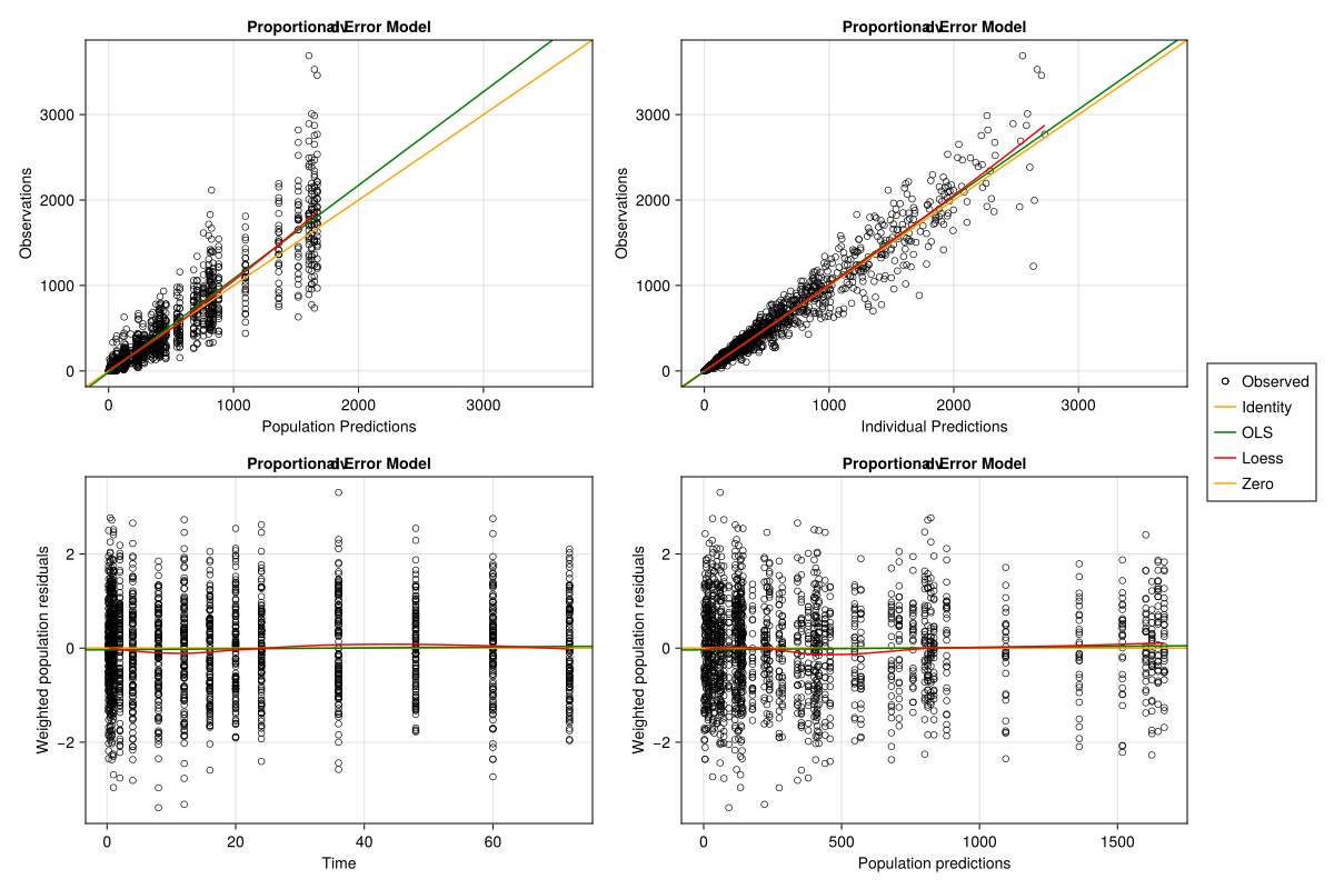
As you can the proportional error model has a lower AIC than the additive, hence it should be preferred.
But let’s take a look at visual diagnostics.
1.5.1.1 Goodness of Fit Plots
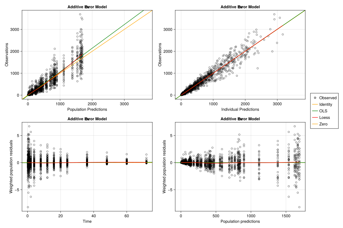
We can pass any result from inspect to the goodness_of_fit plotting function:
goodness_of_fit(
    inspect_proportional;
    figure = (; size = (1200, 800)),
    axis = (; title = "Proportional Error Model"),
)
goodness_of_fit(
    inspect_additive;
    figure = (; size = (1200, 800)),
    axis = (; title = "Additive Error Model"),
)
Tip
We are using some keyword arguments to customize the plot returned by the goodness_of_fit function.
Please check Pumas’ documentation on plot customization for more details.
The weighted residuals should be standard normally distributed throughout the time and the individual predictions domain.
We see that this is the case for the proportional error model, but certainly not for the additive error model. The additive error model weighted residuals’ variance increases with the individual predictions values.
This is another indicator that the additive error model is not able to capture the data generating process.
Tip
One might also plot a QQ plot to check for normality of the residuals.
1.5.2 Visual Predictive Checks (VPCs)
To conclude, we can inspect visual predictive checks with the vpc_plot() function. But first, we need to generate a VPC object with the vpc() function:
vpc_proportional = vpc(fit_proportional)[ Info: Continuous VPC
Visual Predictive Check
  Type of VPC: Continuous VPC
  Simulated populations: 499
  Subjects in data: 120
  Stratification variable(s): None
  Confidence level: 0.95
  VPC lines: quantiles ([0.1, 0.5, 0.9])
vpc_additive = vpc(fit_additive)[ Info: Continuous VPC
Visual Predictive Check
  Type of VPC: Continuous VPC
  Simulated populations: 499
  Subjects in data: 120
  Stratification variable(s): None
  Confidence level: 0.95
  VPC lines: quantiles ([0.1, 0.5, 0.9])
Now, we need to use the vpc_plot function into our newly created VPC object:
vpc_plot(vpc_proportional; axis = (; title = "Proportional Error Model"))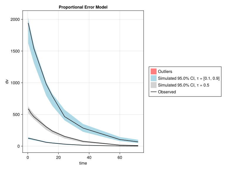
vpc_plot(vpc_additive; axis = (; title = "Additive Error Model"))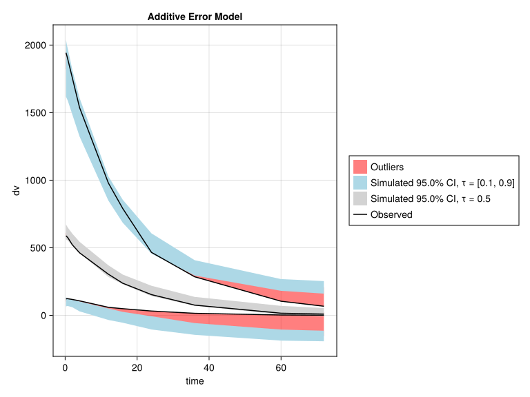
As you can see in the VPC plots above, the additive error model performs poorly in the visual predictive checks, and its quantiles even capture negative concentrations.
Hence, this is the final nail in the coffin of the additive error. Ultimately, we should prefer the proportional error model.
2 Conclusion
This tutorial showed how to use fit a PK model in Pumas and how to compare models.
Please try out fit on your own data and model, and reach out if further questions or problems come up.