using Pumas
using PumasUtilities
using NCA
using NCAUtilities
A Comprehensive Introduction to Pumas
This tutorial provides a comprehensive introduction to a modeling and simulation workflow in Pumas. The idea is not to get into the details of Pumas specifics, but instead provide a narrative on the lines of a regular workflow in our day-to-day work, with brevity where required to allow a broad overview. Wherever possible, cross-references will be provided to documentation and detailed examples that provide deeper insight into a particular topic.
As part of this workflow, you will be introduced to various aspects such as:
- Data wrangling in Julia
- Exploratory analysis in Julia
- Continuous data non-linear mixed effects modeling in Pumas
- Model comparison routines, post-processing, validation etc.
1 The Study and Design
CTMNopain is a novel anti-inflammatory agent under preliminary investigation. A dose-ranging trial was conducted comparing placebo with 3 doses of CTMNopain (5mg, 20mg and 80 mg QD). The maximum tolerated dose is 160 mg per day. Plasma concentrations (mg/L) of the drug were measured at 0, 0.5, 1, 1.5, 2, 2.5, 3-8 hours.
Pain score (0=no pain, 1=mild, 2=moderate, 3=severe) were obtained at time points when plasma concentration was collected. A pain score of 2 or more is considered as no pain relief.
The subjects can request for remedication if pain relief is not achieved after 2 hours post dose. Some subjects had remedication before 2 hours if they were not able to bear the pain. The time to remedication and the remedication status is available for subjects.
The pharmacokinetic dataset can be accessed using PharmaDatasets.jl.
2 Setup
2.1 Load libraries
These libraries provide the workhorse functionality in the Pumas ecosystem:
In addition, libraries below are good add-on’s that provide ancillary functionality:
using GLM: lm, @formula
using Random
using CSV
using DataFramesMeta
using CairoMakie
using PharmaDatasets
2.2 Data Wrangling
We start by reading in the dataset and making some quick summaries.
Tip
If you want to learn more about data wrangling, don’t forget to check our Data Wrangling in Julia tutorials!
pkpain_df = dataset("pk_painrelief")
first(pkpain_df, 5)
5×7 DataFrame
| Row | Subject | Time | Conc | PainRelief | PainScore | RemedStatus | Dose |
|---|---|---|---|---|---|---|---|
| Int64 | Float64 | Float64 | Int64 | Int64 | Int64 | String7 | |
| 1 | 1 | 0.0 | 0.0 | 0 | 3 | 1 | 20 mg |
| 2 | 1 | 0.5 | 1.15578 | 1 | 1 | 0 | 20 mg |
| 3 | 1 | 1.0 | 1.37211 | 1 | 0 | 0 | 20 mg |
| 4 | 1 | 1.5 | 1.30058 | 1 | 0 | 0 | 20 mg |
| 5 | 1 | 2.0 | 1.19195 | 1 | 1 | 0 | 20 mg |
Let’s filter out the placebo data as we don’t need that for the PK analysis.
pkpain_noplb_df = @rsubset pkpain_df :Dose != "Placebo";
first(pkpain_noplb_df, 5)
5×7 DataFrame
| Row | Subject | Time | Conc | PainRelief | PainScore | RemedStatus | Dose |
|---|---|---|---|---|---|---|---|
| Int64 | Float64 | Float64 | Int64 | Int64 | Int64 | String7 | |
| 1 | 1 | 0.0 | 0.0 | 0 | 3 | 1 | 20 mg |
| 2 | 1 | 0.5 | 1.15578 | 1 | 1 | 0 | 20 mg |
| 3 | 1 | 1.0 | 1.37211 | 1 | 0 | 0 | 20 mg |
| 4 | 1 | 1.5 | 1.30058 | 1 | 0 | 0 | 20 mg |
| 5 | 1 | 2.0 | 1.19195 | 1 | 1 | 0 | 20 mg |
3 Analysis
3.1 Non-compartmental analysis
Let’s begin by performing a quick NCA of the concentration time profiles and view the exposure changes across doses. The input data specification for NCA analysis requires the presence of a :route column and an :amt column that specifies the dose. So, let’s add that in:
@rtransform! pkpain_noplb_df begin
    :route = "ev"
    :Dose = parse(Int, chop(:Dose; tail = 3))
end
We also need to create an :amt column:
@rtransform! pkpain_noplb_df :amt = :Time == 0 ? :Dose : missingNow, we map the data variables to the read_nca function that prepares the data for NCA analysis.
pkpain_nca = read_nca(
    pkpain_noplb_df;
    id = :Subject,
    time = :Time,
    amt = :amt,
    observations = :Conc,
    group = [:Dose],
    route = :route,
)
NCAPopulation (120 subjects):
Group: [["Dose" => 5], ["Dose" => 20], ["Dose" => 80]]
Number of missing observations: 0
Number of blq observations: 0Now that we mapped the data in, let’s visualize the concentration vs time plots for a few individuals. When paginate is set to true, a vector of plots are returned and below we display the first element with 9 individuals.
f = observations_vs_time(
    pkpain_nca;
    paginate = true,
    axis = (; xlabel = "Time (hr)", ylabel = "CTMNoPain Concentration (ng/mL)"),
)
f[1]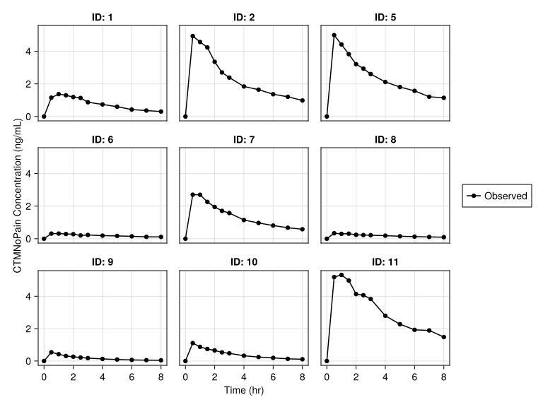
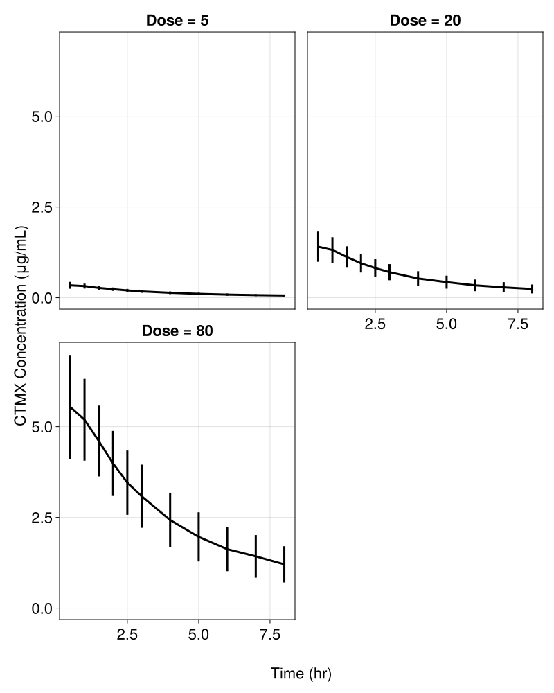
or you can view the summary curves by dose group as passed in to the group argument in read_nca
summary_observations_vs_time(
    pkpain_nca,
    figure = (; fontsize = 22, size = (800, 1000)),
    color = "black",
    linewidth = 3,
    axis = (; xlabel = "Time (hr)", ylabel = "CTMX Concentration (μg/mL)"),
)
A full NCA Report is now obtained for completeness purposes using the run_nca function, but later we will only extract a couple of key metrics of interest.
pk_nca = run_nca(pkpain_nca; sigdigits = 3)We can look at the NCA fits for some subjects. Here f is a vector or figures. We’ll showcase the first image by indexing f:
f = subject_fits(
    pk_nca,
    paginate = true,
    axis = (; xlabel = "Time (hr)", ylabel = "CTMX Concentration (μg/mL)"),

    # Legend options
    legend = (; position = :bottom),
)
f[1]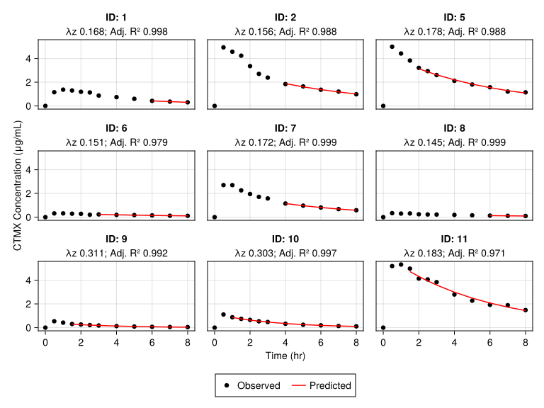
As CTMNopain’s effect maybe mainly related to maximum concentration (cmax) or area under the curve (auc), we present some summary statistics using the summarize function from NCA.
strata = [:Dose]1-element Vector{Symbol}:
:Doseparams = [:cmax, :aucinf_obs]2-element Vector{Symbol}:
:cmax
:aucinf_obsoutput = summarize(pk_nca; stratify_by = strata, parameters = params)6×10 DataFrame
| Row | Dose | parameters | numsamples | minimum | maximum | mean | std | geomean | geostd | geomeanCV |
|---|---|---|---|---|---|---|---|---|---|---|
| Int64 | String | Int64 | Float64 | Float64 | Float64 | Float64 | Float64 | Float64 | Float64 | |
| 1 | 5 | cmax | 40 | 0.19 | 0.539 | 0.356075 | 0.0884129 | 0.345104 | 1.2932 | 26.1425 |
| 2 | 5 | aucinf_obs | 40 | 0.914 | 3.4 | 1.5979 | 0.490197 | 1.53373 | 1.32974 | 29.0868 |
| 3 | 20 | cmax | 40 | 0.933 | 2.7 | 1.4737 | 0.361871 | 1.43408 | 1.2633 | 23.6954 |
| 4 | 20 | aucinf_obs | 40 | 2.77 | 14.1 | 6.377 | 2.22239 | 6.02031 | 1.41363 | 35.6797 |
| 5 | 80 | cmax | 40 | 3.3 | 8.47 | 5.787 | 1.31957 | 5.64164 | 1.25757 | 23.2228 |
| 6 | 80 | aucinf_obs | 40 | 13.7 | 49.1 | 29.5 | 8.68984 | 28.2954 | 1.34152 | 30.0258 |
The statistics printed above are the default, but you can pass in your own statistics using the stats = [] argument to the summarize function.
We can look at a few parameter distribution plots.
parameters_vs_group(
    pk_nca,
    parameter = :cmax,
    axis = (; xlabel = "Dose (mg)", ylabel = "Cₘₐₓ (ng/mL)"),
    figure = (; fontsize = 18),
)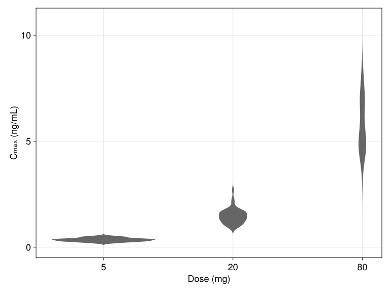
Dose normalized PK parameters, cmax and aucinf were essentially dose proportional between for 5 mg, 20 mg and 80 mg doses. You can perform a simple regression to check the impact of dose on cmax:
dp = NCA.DoseLinearityPowerModel(pk_nca, :cmax; level = 0.9)Dose Linearity Power Model
Variable: cmax
Model: log(cmax) ~ log(α) + β × log(dose)
────────────────────────────────────
Estimate low CI 90% high CI 90%
────────────────────────────────────
β 1.00775 0.97571 1.0398
────────────────────────────────────Here’s a visualization for the dose linearity using a power model for cmax:
power_model(dp; legend = (; position = :bottom))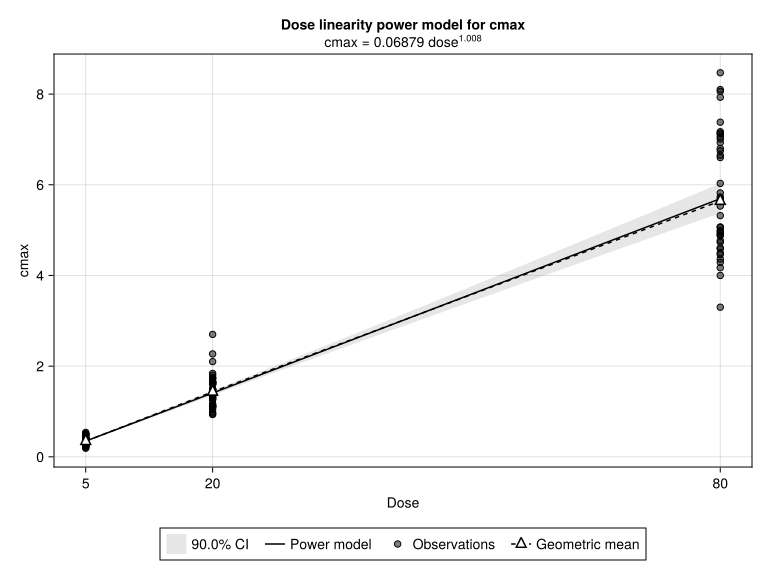
We can also visualize a dose proportionality results with respect to a specific endpoint in a NCA Report; for example cmax and aucinf_obs:
dose_vs_dose_normalized(pk_nca, :cmax)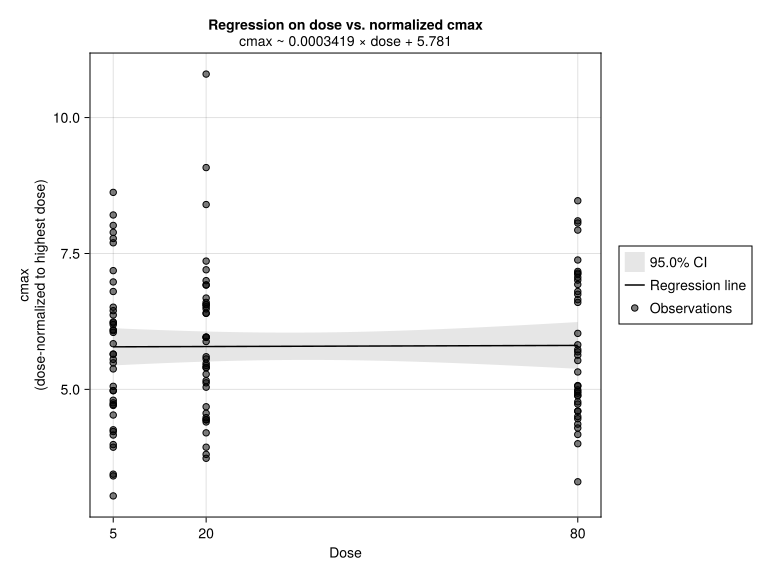
dose_vs_dose_normalized(pk_nca, :aucinf_obs)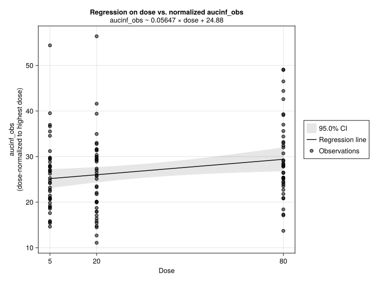
Based on visual inspection of the concentration time profiles as seen earlier, CTMNopain exhibited monophasic decline, and perhaps a one compartment model best fits the PK data.
3.2 Pharmacokinetic modeling
As seen from the plots above, the concentrations decline monoexponentially. We will evaluate both one and two compartment structural models to assess best fit. Further, different residual error models will also be tested.
We will use the results from NCA to provide us good initial estimates.
3.2.1 Data preparation for modeling
PumasNDF requires the presence of :evid and :cmt columns in the dataset.
@rtransform! pkpain_noplb_df begin
    :evid = :Time == 0 ? 1 : 0
    :cmt = :Time == 0 ? 1 : 2
    :cmt2 = 1 # for zero order absorption
end
Further, observations at time of dosing, i.e., when evid = 1 have to be missing
@rtransform! pkpain_noplb_df :Conc = :evid == 1 ? missing : :ConcThe dataframe will now be converted to a Population using read_pumas. Note that both observations and covariates are required to be an array even if it is one element.
pkpain_noplb = read_pumas(
    pkpain_noplb_df;
    id = :Subject,
    time = :Time,
    amt = :amt,
    observations = [:Conc],
    covariates = [:Dose],
    evid = :evid,
    cmt = :cmt,
)
Population
Subjects: 120
Covariates: Dose
Observations: ConcNow that the data is transformed to a Population of subjects, we can explore different models.
3.2.2 One-compartment model
Note
If you are not familiar yet with the @model blocks and syntax, please check our documentation.
pk_1cmp = @model begin

    @metadata begin
        desc = "One Compartment Model"
        timeu = u"hr"
    end

    @param begin
        """
        Clearance (L/hr)
        """
        tvcl ∈ RealDomain(; lower = 0, init = 3.2)
        """
        Volume (L)
        """
        tvv ∈ RealDomain(; lower = 0, init = 16.4)
        """
        Absorption rate constant (h-1)
        """
        tvka ∈ RealDomain(; lower = 0, init = 3.8)
        """
          - ΩCL
          - ΩVc
          - ΩKa
        """
        Ω ∈ PDiagDomain(init = [0.04, 0.04, 0.04])
        """
        Proportional RUV
        """
        σ_p ∈ RealDomain(; lower = 0.0001, init = 0.2)
    end

    @random begin
        η ~ MvNormal(Ω)
    end

    @pre begin
        CL = tvcl * exp(η[1])
        Vc = tvv * exp(η[2])
        Ka = tvka * exp(η[3])
    end

    @dynamics Depots1Central1

    @derived begin
        cp := @. Central / Vc
        """
        CTMx Concentration (ng/mL)
        """
        Conc ~ @. ProportionalNormal(cp, σ_p)
    end

end
PumasModel
Parameters: tvcl, tvv, tvka, Ω, σ_p
Random effects: η
Covariates:
Dynamical system variables: Depot, Central
Dynamical system type: Closed form
Derived: Conc
Observed: Conc
Tip
Note that the local assignment := can be used to define intermediate statements that will not be carried outside of the block. This means that all the resulting data workflows from this model will not contain the intermediate variables defined with :=. We use this when we want to suppress the variable from any further output.
The idea behind := is for performance reasons. If you are not carrying the variable defined with := outside of the block, then it is not necessary to store it in the resulting data structures. Not only will your model run faster, but the resulting data structures will also be smaller.
Before going to fit the model, let’s evaluate some helpful steps via simulation to check appropriateness of data and model
# zero out the random effects
etas = zero_randeffs(pk_1cmp, pkpain_noplb, init_params(pk_1cmp))
Above, we are generating a vector of η’s of the same length as the number of subjects to zero out the random effects. We do this as we are evaluating the trajectories of the concentrations at the initial set of parameters at a population level. Other helper functions here are sample_randeffs and init_randeffs. Please refer to the documentation.
simpk_iparams = simobs(pk_1cmp, pkpain_noplb, init_params(pk_1cmp), etas)Simulated population (Vector{<:Subject})
Simulated subjects: 120
Simulated variables: Concsim_plot(
pk_1cmp,
simpk_iparams;
observations = [:Conc],
figure = (; fontsize = 18),
axis = (;
xlabel = "Time (hr)",
ylabel = "Observed/Predicted \n CTMx Concentration (ng/mL)",
),
)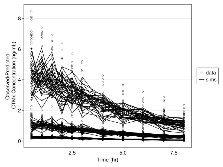
Our NCA based initial guess on the parameters seem to work well.
Lets change the initial estimate of a couple of the parameters to evaluate the sensitivity.
pkparam = (; init_params(pk_1cmp)..., tvka = 2, tvv = 10)(tvcl = 3.2, tvv = 10, tvka = 2, Ω = [0.04 0.0 0.0; 0.0 0.04 0.0; 0.0 0.0 0.04], σ_p = 0.2)simpk_changedpars = simobs(pk_1cmp, pkpain_noplb, pkparam, etas)Simulated population (Vector{<:Subject})
Simulated subjects: 120
Simulated variables: Concsim_plot(
pk_1cmp,
simpk_changedpars;
observations = [:Conc],
figure = (; fontsize = 18),
axis = (
xlabel = "Time (hr)",
ylabel = "Observed/Predicted \n CTMx Concentration (ng/mL)",
),
)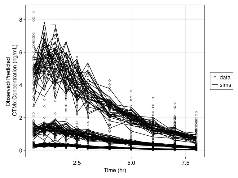
Changing the tvka and decreasing the tvv seemed to make an impact and observations go through the simulated lines.
To get a quick ballpark estimate of your PK parameters, we can do a NaivePooled analysis.
3.2.2.1 NaivePooled
pkparam_np = (; init_params(pk_1cmp)..., Ω = Diagonal(zeros(3)))
pkfit_np = fit(pk_1cmp, pkpain_noplb, pkparam_np, NaivePooled(); constantcoef = (:Ω,))
[ Info: Checking the initial parameter values. [ Info: The initial negative log likelihood and its gradient are finite. Check passed. Iter Function value Gradient norm 0 7.744356e+02 3.715711e+03 * time: 0.05212712287902832 1 2.343899e+02 1.747348e+03 * time: 2.88360595703125 2 9.696232e+01 1.198088e+03 * time: 2.8913381099700928 3 -7.818699e+01 5.538151e+02 * time: 2.8972089290618896 4 -1.234803e+02 2.462514e+02 * time: 2.902949094772339 5 -1.372888e+02 2.067458e+02 * time: 2.906604051589966 6 -1.410579e+02 1.162950e+02 * time: 2.9095780849456787 7 -1.434754e+02 5.632816e+01 * time: 2.9123549461364746 8 -1.453401e+02 7.859270e+01 * time: 2.915092945098877 9 -1.498185e+02 1.455606e+02 * time: 2.917794942855835 10 -1.534371e+02 1.303682e+02 * time: 2.920586109161377 11 -1.563557e+02 5.975474e+01 * time: 2.9233760833740234 12 -1.575052e+02 9.308611e+00 * time: 2.926007032394409 13 -1.579357e+02 1.234484e+01 * time: 2.9286139011383057 14 -1.581874e+02 7.478196e+00 * time: 2.931175947189331 15 -1.582981e+02 2.027162e+00 * time: 2.933756113052368 16 -1.583375e+02 5.578262e+00 * time: 2.936264991760254 17 -1.583556e+02 4.727050e+00 * time: 2.938767910003662 18 -1.583644e+02 2.340173e+00 * time: 2.9414010047912598 19 -1.583680e+02 7.738100e-01 * time: 2.9440650939941406 20 -1.583696e+02 3.300689e-01 * time: 2.9466769695281982 21 -1.583704e+02 3.641985e-01 * time: 2.9496209621429443 22 -1.583707e+02 4.365901e-01 * time: 2.952263116836548 23 -1.583709e+02 3.887800e-01 * time: 2.9549129009246826 24 -1.583710e+02 2.766977e-01 * time: 2.957534074783325 25 -1.583710e+02 1.758029e-01 * time: 2.9601850509643555 26 -1.583710e+02 1.133947e-01 * time: 2.962738037109375 27 -1.583710e+02 7.922544e-02 * time: 2.9653820991516113 28 -1.583710e+02 5.954998e-02 * time: 2.9680418968200684 29 -1.583710e+02 4.157080e-02 * time: 2.9707000255584717 30 -1.583710e+02 4.295446e-02 * time: 2.973357915878296 31 -1.583710e+02 5.170752e-02 * time: 2.9760239124298096 32 -1.583710e+02 2.644382e-02 * time: 2.9798810482025146 33 -1.583710e+02 4.548987e-03 * time: 2.983755111694336 34 -1.583710e+02 2.501806e-02 * time: 2.9879400730133057 35 -1.583710e+02 3.763439e-02 * time: 2.990614891052246 36 -1.583710e+02 3.206026e-02 * time: 2.9931740760803223 37 -1.583710e+02 1.003701e-02 * time: 2.995758056640625 38 -1.583710e+02 2.209083e-02 * time: 2.998353958129883 39 -1.583710e+02 4.954121e-03 * time: 3.0021679401397705 40 -1.583710e+02 1.609362e-02 * time: 3.006127119064331 41 -1.583710e+02 1.579815e-02 * time: 3.0087339878082275 42 -1.583710e+02 1.014181e-03 * time: 3.0113940238952637 43 -1.583710e+02 6.050877e-03 * time: 3.015413999557495 44 -1.583710e+02 1.354363e-02 * time: 3.018091917037964 45 -1.583710e+02 4.473198e-03 * time: 3.0207650661468506 46 -1.583710e+02 4.645873e-03 * time: 3.0236220359802246 47 -1.583710e+02 9.827001e-03 * time: 3.026308059692383 48 -1.583710e+02 1.047016e-03 * time: 3.029093027114868 49 -1.583710e+02 8.378247e-03 * time: 3.031709909439087 50 -1.583710e+02 7.820745e-04 * time: 3.0344479084014893
FittedPumasModel

Dynamical system type:                 Closed form

Number of subjects:                            120

Observation records:         Active        Missing
    Conc:                      1320              0
    Total:                     1320              0

Number of parameters:      Constant      Optimized
                                  1              6

Likelihood approximation:              NaivePooled
Likelihood optimizer:                         BFGS

Termination Reason:                   GradientNorm
Log-likelihood value:                    158.37103

------------------
         Estimate
------------------
  tvcl    3.0054
  tvv    14.089
  tvka   44.227
† Ω₁,₁    0.0
† Ω₂,₂    0.0
† Ω₃,₃    0.0
  σ_p     0.32999
------------------
† indicates constant parameterscoefficients_table(pkfit_np)7×4 DataFrame
| Row | Parameter | Description | Constant | Estimate |
|---|---|---|---|---|
| String | SubStrin… | Bool | Float64 | |
| 1 | tvcl | Clearance (L/hr) | false | 3.005 |
| 2 | tvv | Volume (L) | false | 14.089 |
| 3 | tvka | Absorption rate constant (h-1) | false | 44.227 |
| 4 | Ω₁,₁ | ΩCL | true | 0.0 |
| 5 | Ω₂,₂ | ΩVc | true | 0.0 |
| 6 | Ω₃,₃ | ΩKa | true | 0.0 |
| 7 | σ_p | Proportional RUV | false | 0.33 |
The final estimates from the NaivePooled approach seem reasonably close to our initial guess from NCA, except for the tvka parameter. We will stick with our initial guess.
One way to be cautious before going into a complete fitting routine is to evaluate the likelihood of the individual subjects given the initial parameter values and see if any subject(s) pops out as unreasonable. There are a few ways of doing this:
- check the
loglikelihoodsubject wise - check if there any influential subjects
Below, we are basically checking if the initial estimates for any subject are way off that we are unable to compute the initial loglikelihood.
lls = [loglikelihood(pk_1cmp, subj, pkparam, FOCE()) for subj in pkpain_noplb]
# the plot below is using native CairoMakie `hist`
hist(lls; bins = 10, normalization = :none, color = (:black, 0.5))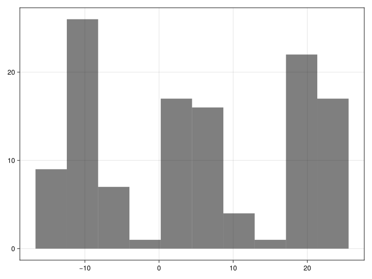
The distribution of the loglikelihood’s suggest no extreme outliers.
A more convenient way is to use the findinfluential function that provides a list of k top influential subjects by showing the normalized (minus) loglikelihood for each subject. As you can see below, the minus loglikelihood in the range of 16 agrees with the histogram plotted above.
influential_subjects = findinfluential(pk_1cmp, pkpain_noplb, pkparam, FOCE())120-element Vector{@NamedTuple{id::String, nll::Float64}}:
(id = "148", nll = 16.659658856844782)
(id = "135", nll = 16.648985190076324)
(id = "156", nll = 15.9590695566075)
(id = "159", nll = 15.441218240496484)
(id = "149", nll = 14.715134644119514)
(id = "88", nll = 13.09709837464614)
(id = "16", nll = 12.982280521931417)
(id = "61", nll = 12.652182902303675)
(id = "71", nll = 12.500330088085486)
(id = "59", nll = 12.241510254805224)
⋮
(id = "57", nll = -22.797674232534305)
(id = "93", nll = -22.836900711478222)
(id = "12", nll = -23.007742339519236)
(id = "123", nll = -23.292751843079227)
(id = "41", nll = -23.425412534960515)
(id = "99", nll = -23.53521484190102)
(id = "29", nll = -24.025959868383097)
(id = "52", nll = -24.164757842493685)
(id = "24", nll = -25.572092325658446)3.2.2.2 FOCE
Now that we have a good handle on our data, lets go ahead and fit a population model with FOCE:
pkfit_1cmp = fit(pk_1cmp, pkpain_noplb, pkparam, FOCE(); constantcoef = (:tvka,))[ Info: Checking the initial parameter values. [ Info: The initial negative log likelihood and its gradient are finite. Check passed. Iter Function value Gradient norm 0 -5.935351e+02 5.597318e+02 * time: 4.315376281738281e-5 1 -7.022088e+02 1.707063e+02 * time: 1.3439180850982666 2 -7.314067e+02 2.903269e+02 * time: 1.9727401733398438 3 -8.520591e+02 2.285888e+02 * time: 2.0970540046691895 4 -1.120191e+03 3.795410e+02 * time: 2.8438611030578613 5 -1.178784e+03 2.323978e+02 * time: 2.9694371223449707 6 -1.218320e+03 9.699907e+01 * time: 3.144700050354004 7 -1.223641e+03 5.862105e+01 * time: 3.2392141819000244 8 -1.227620e+03 1.831402e+01 * time: 3.334635019302368 9 -1.228381e+03 2.132323e+01 * time: 3.4623332023620605 10 -1.230098e+03 2.921228e+01 * time: 3.5559561252593994 11 -1.230854e+03 2.029661e+01 * time: 3.6452460289001465 12 -1.231116e+03 5.229104e+00 * time: 3.7324471473693848 13 -1.231179e+03 1.689231e+00 * time: 3.848294973373413 14 -1.231187e+03 1.215378e+00 * time: 3.9315381050109863 15 -1.231188e+03 2.770380e-01 * time: 4.0089640617370605 16 -1.231188e+03 1.636651e-01 * time: 4.107218027114868 17 -1.231188e+03 2.701104e-01 * time: 4.176918983459473 18 -1.231188e+03 3.163369e-01 * time: 4.2454609870910645 19 -1.231188e+03 1.505174e-01 * time: 4.312628984451294 20 -1.231188e+03 2.484690e-02 * time: 4.417344093322754 21 -1.231188e+03 8.387527e-04 * time: 4.477440118789673
FittedPumasModel

Dynamical system type:                 Closed form

Number of subjects:                            120

Observation records:         Active        Missing
    Conc:                      1320              0
    Total:                     1320              0

Number of parameters:      Constant      Optimized
                                  1              6

Likelihood approximation:                     FOCE
Likelihood optimizer:                         BFGS

Termination Reason:                   GradientNorm
Log-likelihood value:                     1231.188

-------------------
         Estimate
-------------------
  tvcl    3.1642
  tvv    13.288
† tvka    2.0
  Ω₁,₁    0.08494
  Ω₂,₂    0.048568
  Ω₃,₃    5.5811
  σ_p     0.10093
-------------------
† indicates constant parametersinfer(pkfit_1cmp)[ Info: Calculating: variance-covariance matrix. [ Info: Done.
Asymptotic inference results using sandwich estimator

Dynamical system type:                 Closed form

Number of subjects:                            120

Observation records:         Active        Missing
    Conc:                      1320              0
    Total:                     1320              0

Number of parameters:      Constant      Optimized
                                  1              6

Likelihood approximation:                     FOCE
Likelihood optimizer:                         BFGS

Termination Reason:                   GradientNorm
Log-likelihood value:                     1231.188

---------------------------------------------------------
         Estimate    SE          95.0% C.I.
---------------------------------------------------------
  tvcl    3.1642     0.08662     [  2.9944  ;  3.334   ]
  tvv    13.288      0.27481     [ 12.749   ; 13.827   ]
† tvka    2.0        NaN         [  NaN     ;  NaN     ]
  Ω₁,₁    0.08494    0.011022    [  0.063338;  0.10654 ]
  Ω₂,₂    0.048568   0.0063502   [  0.036122;  0.061014]
  Ω₃,₃    5.5811     1.2188      [  3.1922  ;  7.97    ]
  σ_p     0.10093    0.0057196   [  0.089718;  0.11214 ]
---------------------------------------------------------
† indicates constant parameters
Notice that tvka is fixed to 2 as we don’t have a lot of information before tmax. From the results above, we see that the parameter precision for this model is reasonable.
3.2.3 Two-compartment model
Just to be sure, let’s fit a 2-compartment model and evaluate:
pk_2cmp = @model begin

    @param begin
        """
        Clearance (L/hr)
        """
        tvcl ∈ RealDomain(; lower = 0, init = 3.2)
        """
        Central Volume (L)
        """
        tvv ∈ RealDomain(; lower = 0, init = 16.4)
        """
        Peripheral Volume (L)
        """
        tvvp ∈ RealDomain(; lower = 0, init = 10)
        """
        Distributional Clearance (L/hr)
        """
        tvq ∈ RealDomain(; lower = 0, init = 2)
        """
        Absorption rate constant (h-1)
        """
        tvka ∈ RealDomain(; lower = 0, init = 1.3)
        """
          - ΩCL
          - ΩVc
          - ΩKa
          - ΩVp
          - ΩQ
        """
        Ω ∈ PDiagDomain(init = [0.04, 0.04, 0.04, 0.04, 0.04])
        """
        Proportional RUV
        """
        σ_p ∈ RealDomain(; lower = 0.0001, init = 0.2)
    end

    @random begin
        η ~ MvNormal(Ω)
    end

    @pre begin
        CL = tvcl * exp(η[1])
        Vc = tvv * exp(η[2])
        Ka = tvka * exp(η[3])
        Vp = tvvp * exp(η[4])
        Q = tvq * exp(η[5])
    end

    @dynamics Depots1Central1Periph1

    @derived begin
        cp := @. Central / Vc
        """
        CTMx Concentration (ng/mL)
        """
        Conc ~ @. ProportionalNormal(cp, σ_p)
    end
end
PumasModel
Parameters: tvcl, tvv, tvvp, tvq, tvka, Ω, σ_p
Random effects: η
Covariates:
Dynamical system variables: Depot, Central, Peripheral
Dynamical system type: Closed form
Derived: Conc
Observed: Conc3.2.3.1 FOCE
pkfit_2cmp = fit(
    pk_2cmp,
    pkpain_noplb,
    (; init_params(pk_2cmp)..., tvka = 2),
    FOCE();
    constantcoef = (:tvka,),
)
[ Info: Checking the initial parameter values. [ Info: The initial negative log likelihood and its gradient are finite. Check passed. Iter Function value Gradient norm 0 -6.302369e+02 1.021050e+03 * time: 2.6941299438476562e-5 1 -9.197817e+02 9.927951e+02 * time: 2.012556791305542 2 -1.372640e+03 2.054986e+02 * time: 4.434926986694336 3 -1.446326e+03 1.543987e+02 * time: 4.809306859970093 4 -1.545570e+03 1.855028e+02 * time: 5.053077936172485 5 -1.581449e+03 1.713157e+02 * time: 5.3997578620910645 6 -1.639433e+03 1.257382e+02 * time: 5.700730800628662 7 -1.695964e+03 7.450539e+01 * time: 5.919094800949097 8 -1.722243e+03 5.961044e+01 * time: 6.210327863693237 9 -1.736883e+03 7.320921e+01 * time: 6.425978899002075 10 -1.753547e+03 7.501938e+01 * time: 6.683363914489746 11 -1.764053e+03 6.185661e+01 * time: 6.908169984817505 12 -1.778991e+03 4.831033e+01 * time: 7.1707680225372314 13 -1.791492e+03 4.943278e+01 * time: 7.442131996154785 14 -1.799847e+03 2.871410e+01 * time: 7.723223924636841 15 -1.805374e+03 7.520790e+01 * time: 8.004272937774658 16 -1.816260e+03 2.990621e+01 * time: 8.277647972106934 17 -1.818252e+03 2.401915e+01 * time: 8.539836883544922 18 -1.822988e+03 2.587225e+01 * time: 8.799099922180176 19 -1.824653e+03 1.550517e+01 * time: 9.04474687576294 20 -1.826074e+03 1.788927e+01 * time: 9.290105819702148 21 -1.826821e+03 1.888389e+01 * time: 9.534603834152222 22 -1.827900e+03 1.432840e+01 * time: 9.78224802017212 23 -1.828511e+03 9.422040e+00 * time: 10.035881996154785 24 -1.828754e+03 5.363445e+00 * time: 10.298183917999268 25 -1.828862e+03 4.916168e+00 * time: 10.55214786529541 26 -1.829007e+03 4.695750e+00 * time: 10.80371880531311 27 -1.829358e+03 1.090244e+01 * time: 11.086951971054077 28 -1.829830e+03 1.451320e+01 * time: 11.354781866073608 29 -1.830201e+03 1.108695e+01 * time: 11.619431018829346 30 -1.830360e+03 2.892317e+00 * time: 11.879026889801025 31 -1.830390e+03 1.699266e+00 * time: 12.158126831054688 32 -1.830404e+03 1.602222e+00 * time: 12.412798881530762 33 -1.830432e+03 2.823465e+00 * time: 12.655174970626831 34 -1.830475e+03 4.119061e+00 * time: 12.91043996810913 35 -1.830527e+03 5.081976e+00 * time: 13.16716480255127 36 -1.830591e+03 2.669398e+00 * time: 13.452636003494263 37 -1.830615e+03 3.513273e+00 * time: 13.704190969467163 38 -1.830623e+03 2.267944e+00 * time: 13.950793981552124 39 -1.830625e+03 1.664224e+00 * time: 14.190936803817749 40 -1.830627e+03 9.587510e-01 * time: 14.436469793319702 41 -1.830628e+03 9.090960e-01 * time: 14.685014009475708 42 -1.830628e+03 3.474532e-01 * time: 14.918846845626831 43 -1.830629e+03 4.588056e-01 * time: 15.148240804672241 44 -1.830630e+03 6.648434e-01 * time: 15.349830865859985 45 -1.830630e+03 4.414323e-01 * time: 15.586055994033813 46 -1.830630e+03 7.962199e-02 * time: 15.807204961776733 47 -1.830630e+03 7.027626e-02 * time: 16.067646980285645 48 -1.830630e+03 2.999926e-02 * time: 16.32205581665039 49 -1.830630e+03 2.754764e-03 * time: 16.52831196784973 50 -1.830630e+03 2.754816e-03 * time: 16.785082817077637 51 -1.830630e+03 2.754867e-03 * time: 17.039378881454468 52 -1.830630e+03 2.754919e-03 * time: 17.31322479248047 53 -1.830630e+03 2.754970e-03 * time: 17.56937599182129 54 -1.830630e+03 2.755022e-03 * time: 17.81862783432007 55 -1.830630e+03 2.755073e-03 * time: 18.070774793624878 56 -1.830630e+03 2.755124e-03 * time: 18.335404872894287 57 -1.830630e+03 2.755129e-03 * time: 18.620059967041016 58 -1.830630e+03 2.755135e-03 * time: 18.915838956832886 59 -1.830630e+03 2.755140e-03 * time: 19.18964385986328 60 -1.830630e+03 2.755145e-03 * time: 19.461131811141968 61 -1.830630e+03 2.755145e-03 * time: 19.733717918395996 62 -1.830630e+03 2.755146e-03 * time: 20.031575918197632 63 -1.830630e+03 2.755146e-03 * time: 20.30859684944153 64 -1.830630e+03 2.755147e-03 * time: 20.584460020065308 65 -1.830630e+03 2.755147e-03 * time: 20.859195947647095 66 -1.830630e+03 2.755148e-03 * time: 21.15712285041809 67 -1.830630e+03 2.755149e-03 * time: 21.43312096595764 68 -1.830630e+03 2.755149e-03 * time: 21.703367948532104 69 -1.830630e+03 2.755150e-03 * time: 21.974844932556152 70 -1.830630e+03 2.755150e-03 * time: 22.280804872512817 71 -1.830630e+03 2.755150e-03 * time: 22.582852840423584 72 -1.830630e+03 2.755150e-03 * time: 22.895335912704468
FittedPumasModel

Dynamical system type:                 Closed form

Number of subjects:                            120

Observation records:         Active        Missing
    Conc:                      1320              0
    Total:                     1320              0

Number of parameters:      Constant      Optimized
                                  1             10

Likelihood approximation:                     FOCE
Likelihood optimizer:                         BFGS

Termination Reason:              NoObjectiveChange
Log-likelihood value:                    1830.6305

-------------------
         Estimate
-------------------
  tvcl    2.8138
  tvv    11.005
  tvvp    5.54
  tvq     1.5159
† tvka    2.0
  Ω₁,₁    0.10267
  Ω₂,₂    0.060776
  Ω₃,₃    1.2012
  Ω₄,₄    0.42349
  Ω₅,₅    0.24473
  σ_p     0.048405
-------------------
† indicates constant parameters
3.3 Comparing One- versus Two-compartment models
The 2-compartment model has a much lower objective function compared to the 1-compartment. Let’s compare the estimates from the 2 models using the compare_estimates function.
compare_estimates(; pkfit_1cmp, pkfit_2cmp)11×3 DataFrame
| Row | parameter | pkfit_1cmp | pkfit_2cmp |
|---|---|---|---|
| String | Float64? | Float64? | |
| 1 | tvcl | 3.1642 | 2.81378 |
| 2 | tvv | 13.288 | 11.0046 |
| 3 | tvka | 2.0 | 2.0 |
| 4 | Ω₁,₁ | 0.0849405 | 0.102669 |
| 5 | Ω₂,₂ | 0.0485682 | 0.0607757 |
| 6 | Ω₃,₃ | 5.58107 | 1.20115 |
| 7 | σ_p | 0.100928 | 0.0484049 |
| 8 | tvvp | missing | 5.53998 |
| 9 | tvq | missing | 1.51591 |
| 10 | Ω₄,₄ | missing | 0.423494 |
| 11 | Ω₅,₅ | missing | 0.244731 |
We perform a likelihood ratio test to compare the two nested models. The test statistic and the \(p\)-value clearly indicate that a 2-compartment model should be preferred.
lrtest(pkfit_1cmp, pkfit_2cmp)Statistic: 1200.0
Degrees of freedom: 4
P-value: 0.0We should also compare the other metrics and statistics, such ηshrinkage, ϵshrinkage, aic, and bic using the metrics_table function.
@chain metrics_table(pkfit_2cmp) begin
    leftjoin(metrics_table(pkfit_1cmp); on = :Metric, makeunique = true)
    rename!(:Value => :pk2cmp, :Value_1 => :pk1cmp)
end
WARNING: using deprecated binding Distributions.MatrixReshaped in Pumas.
, use Distributions.ReshapedDistribution{2, S, D} where D<:Distributions.Distribution{Distributions.ArrayLikeVariate{1}, S} where S<:Distributions.ValueSupport instead.20×3 DataFrame
| Row | Metric | pk2cmp | pk1cmp |
|---|---|---|---|
| String | Any | Any | |
| 1 | Successful | true | true |
| 2 | Estimation Time | 22.895 | 4.478 |
| 3 | Subjects | 120 | 120 |
| 4 | Fixed Parameters | 1 | 1 |
| 5 | Optimized Parameters | 10 | 6 |
| 6 | Conc Active Observations | 1320 | 1320 |
| 7 | Conc Missing Observations | 0 | 0 |
| 8 | Total Active Observations | 1320 | 1320 |
| 9 | Total Missing Observations | 0 | 0 |
| 10 | Likelihood Approximation | Pumas.FOCE{Optim.NewtonTrustRegion{Float64}, Optim.Options{Float64, Nothing}} | Pumas.FOCE{Optim.NewtonTrustRegion{Float64}, Optim.Options{Float64, Nothing}} |
| 11 | LogLikelihood (LL) | 1830.63 | 1231.19 |
| 12 | -2LL | -3661.26 | -2462.38 |
| 13 | AIC | -3641.26 | -2450.38 |
| 14 | BIC | -3589.41 | -2419.26 |
| 15 | (η-shrinkage) η₁ | 0.037 | 0.016 |
| 16 | (η-shrinkage) η₂ | 0.047 | 0.04 |
| 17 | (η-shrinkage) η₃ | 0.516 | 0.733 |
| 18 | (ϵ-shrinkage) Conc | 0.185 | 0.105 |
| 19 | (η-shrinkage) η₄ | 0.287 | missing |
| 20 | (η-shrinkage) η₅ | 0.154 | missing |
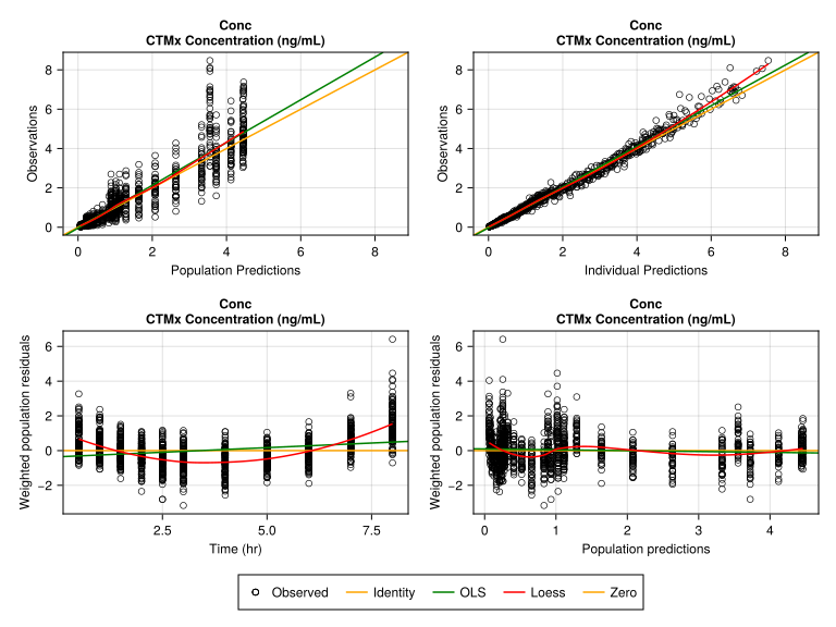
We next generate some goodness of fit plots to compare which model is performing better. To do this, we first inspect the diagnostics of our model fit.
res_inspect_1cmp = inspect(pkfit_1cmp)[ Info: Calculating predictions. [ Info: Calculating weighted residuals. [ Info: Calculating empirical bayes. [ Info: Evaluating dose control parameters. [ Info: Evaluating individual parameters. [ Info: Done.
FittedPumasModelInspection

Likelihood approximation used for weighted residuals: FOCE
res_inspect_2cmp = inspect(pkfit_2cmp)[ Info: Calculating predictions. [ Info: Calculating weighted residuals. [ Info: Calculating empirical bayes. [ Info: Evaluating dose control parameters. [ Info: Evaluating individual parameters. [ Info: Done.
FittedPumasModelInspection

Likelihood approximation used for weighted residuals: FOCE
gof_1cmp = goodness_of_fit(
res_inspect_1cmp;
figure = (; fontsize = 12),
legend = (; position = :bottom),
)
gof_2cmp = goodness_of_fit(
    res_inspect_2cmp;
    figure = (; fontsize = 12),
    legend = (; position = :bottom),
)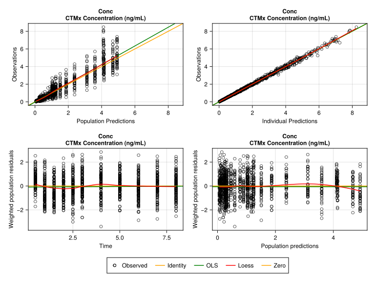
These plots clearly indicate that the 2-compartment model is a better fit compared to the 1-compartment model.
We can look at selected sample of individual plots.
fig_subject_fits = subject_fits(
    res_inspect_2cmp;
    separate = true,
    paginate = true,
    figure = (; fontsize = 18),
    axis = (; xlabel = "Time (hr)", ylabel = "CTMx Concentration (ng/mL)"),
)
fig_subject_fits[1]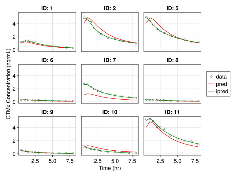
There a lot of important plotting functions you can use for your standard model diagnostics. Please make sure to read the documentation for plotting. Below, we are checking the distribution of the empirical Bayes estimates.
empirical_bayes_dist(res_inspect_2cmp; zeroline_color = :red)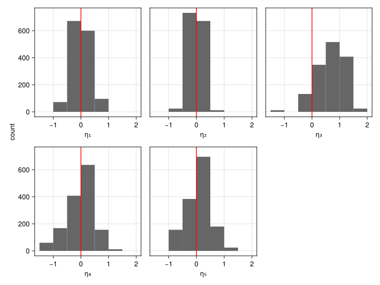
empirical_bayes_vs_covariates(
    res_inspect_2cmp;
    categorical = [:Dose],
    figure = (; size = (600, 800)),
)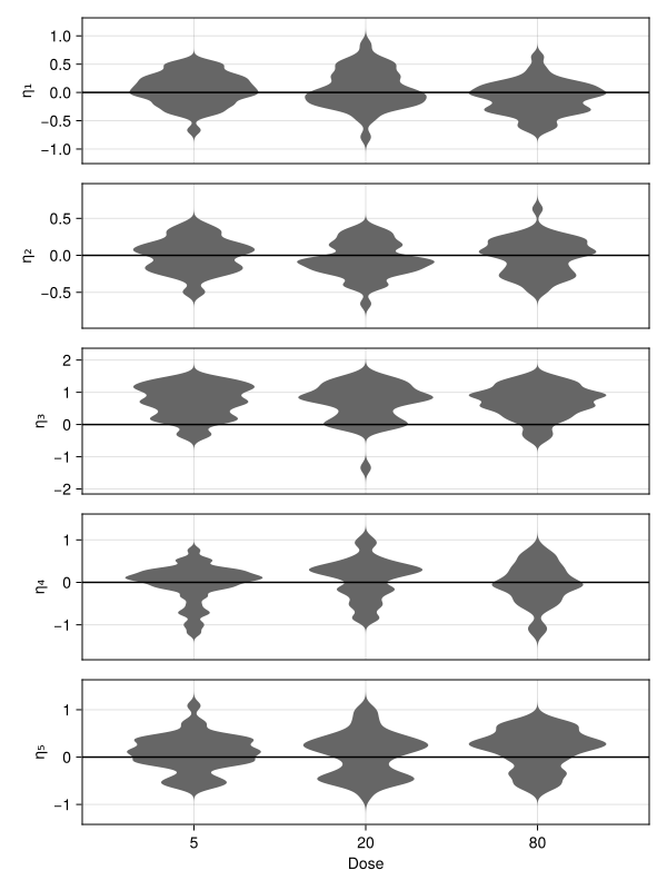
Clearly, our guess at tvka seems off-target. Let’s try and estimate tvka instead of fixing it to 2:
pkfit_2cmp_unfix_ka = fit(pk_2cmp, pkpain_noplb, init_params(pk_2cmp), FOCE())[ Info: Checking the initial parameter values. [ Info: The initial negative log likelihood and its gradient are finite. Check passed. Iter Function value Gradient norm 0 -3.200734e+02 1.272671e+03 * time: 1.5020370483398438e-5 1 -8.682982e+02 1.000199e+03 * time: 1.372908115386963 2 -1.381870e+03 5.008081e+02 * time: 4.2922210693359375 3 -1.551053e+03 6.833490e+02 * time: 4.631515979766846 4 -1.680887e+03 1.834586e+02 * time: 4.937623977661133 5 -1.726118e+03 8.870274e+01 * time: 5.332730054855347 6 -1.761023e+03 1.162036e+02 * time: 5.587187051773071 7 -1.786619e+03 1.114552e+02 * time: 5.852047920227051 8 -1.863556e+03 9.914305e+01 * time: 6.186362028121948 9 -1.882942e+03 5.342676e+01 * time: 6.444565057754517 10 -1.888020e+03 2.010181e+01 * time: 6.732893943786621 11 -1.889832e+03 1.867263e+01 * time: 7.0293121337890625 12 -1.891649e+03 1.668512e+01 * time: 7.310096025466919 13 -1.892615e+03 1.820701e+01 * time: 7.585663080215454 14 -1.893453e+03 1.745195e+01 * time: 7.859210014343262 15 -1.894760e+03 1.850174e+01 * time: 8.133930921554565 16 -1.895647e+03 1.773939e+01 * time: 8.404133081436157 17 -1.896597e+03 1.143462e+01 * time: 8.669528007507324 18 -1.897114e+03 9.720097e+00 * time: 8.938102006912231 19 -1.897373e+03 6.054321e+00 * time: 9.20905613899231 20 -1.897498e+03 3.985954e+00 * time: 9.479493141174316 21 -1.897571e+03 4.262464e+00 * time: 9.739084005355835 22 -1.897633e+03 4.010234e+00 * time: 10.005645036697388 23 -1.897714e+03 4.805375e+00 * time: 10.264682054519653 24 -1.897802e+03 3.508706e+00 * time: 10.533371925354004 25 -1.897865e+03 3.691475e+00 * time: 10.799684047698975 26 -1.897900e+03 2.982721e+00 * time: 11.067280054092407 27 -1.897928e+03 2.563790e+00 * time: 11.326159000396729 28 -1.897968e+03 3.261485e+00 * time: 11.588170051574707 29 -1.898013e+03 3.064689e+00 * time: 11.847042083740234 30 -1.898040e+03 1.636525e+00 * time: 12.118109941482544 31 -1.898051e+03 1.439997e+00 * time: 12.38301706314087 32 -1.898057e+03 1.436504e+00 * time: 12.648709058761597 33 -1.898069e+03 1.881528e+00 * time: 12.9199800491333 34 -1.898095e+03 3.253164e+00 * time: 13.189949035644531 35 -1.898142e+03 4.257941e+00 * time: 13.461146116256714 36 -1.898199e+03 3.685241e+00 * time: 13.759012937545776 37 -1.898245e+03 2.567364e+00 * time: 14.041224956512451 38 -1.898246e+03 2.561569e+00 * time: 14.4411780834198 39 -1.898251e+03 2.530909e+00 * time: 15.07192611694336 40 -1.898298e+03 2.673535e+00 * time: 15.454133033752441 41 -1.898300e+03 2.796024e+00 * time: 15.831545114517212 42 -1.898337e+03 3.655512e+00 * time: 16.241007089614868 43 -1.898342e+03 3.773931e+00 * time: 16.713839054107666 44 -1.898433e+03 4.520984e+00 * time: 17.09260392189026 45 -1.898463e+03 3.636788e+00 * time: 17.36982011795044 46 -1.898477e+03 2.415944e+00 * time: 17.686872959136963 47 -1.898479e+03 1.827052e+00 * time: 18.006355047225952 48 -1.898479e+03 5.288379e-01 * time: 18.3493709564209 49 -1.898479e+03 4.636056e-01 * time: 18.71838092803955 50 -1.898480e+03 1.435316e+00 * time: 19.004637956619263 51 -1.898480e+03 2.491286e+00 * time: 19.29581594467163 52 -1.898480e+03 1.103596e-01 * time: 19.63326406478882 53 -1.898480e+03 4.098989e-02 * time: 19.875908136367798 54 -1.898480e+03 4.098989e-02 * time: 20.230085134506226 55 -1.898480e+03 4.098989e-02 * time: 20.668843984603882 56 -1.898480e+03 4.098989e-02 * time: 21.084005117416382 57 -1.898480e+03 5.127712e-03 * time: 21.36496615409851 58 -1.898480e+03 5.152593e-03 * time: 21.625606060028076 59 -1.898480e+03 5.152815e-03 * time: 21.908765077590942 60 -1.898480e+03 5.153036e-03 * time: 22.22110605239868 61 -1.898480e+03 5.153059e-03 * time: 22.549122095108032 62 -1.898480e+03 5.153081e-03 * time: 22.854114055633545 63 -1.898480e+03 5.153103e-03 * time: 23.16753101348877 64 -1.898480e+03 5.153125e-03 * time: 23.468585968017578 65 -1.898480e+03 5.153147e-03 * time: 23.798710107803345 66 -1.898480e+03 5.153169e-03 * time: 24.10114812850952 67 -1.898480e+03 5.153192e-03 * time: 24.394386053085327 68 -1.898480e+03 5.153194e-03 * time: 24.692012071609497 69 -1.898480e+03 5.153196e-03 * time: 24.993396043777466 70 -1.898480e+03 5.153198e-03 * time: 25.31931495666504 71 -1.898480e+03 5.153200e-03 * time: 25.625257968902588 72 -1.898480e+03 5.153203e-03 * time: 25.923567056655884 73 -1.898480e+03 5.153205e-03 * time: 26.226294994354248 74 -1.898480e+03 5.153207e-03 * time: 26.57996702194214 75 -1.898480e+03 5.153209e-03 * time: 26.8821439743042 76 -1.898480e+03 5.153212e-03 * time: 27.1879141330719 77 -1.898480e+03 5.153212e-03 * time: 27.50110411643982 78 -1.898480e+03 5.153212e-03 * time: 27.847574949264526 79 -1.898480e+03 5.153212e-03 * time: 28.20265793800354 80 -1.898480e+03 5.153212e-03 * time: 28.62150502204895 81 -1.898480e+03 5.153212e-03 * time: 29.021700143814087
FittedPumasModel

Dynamical system type:                 Closed form

Number of subjects:                            120

Observation records:         Active        Missing
    Conc:                      1320              0
    Total:                     1320              0

Number of parameters:      Constant      Optimized
                                  0             11

Likelihood approximation:                     FOCE
Likelihood optimizer:                         BFGS

Termination Reason:              NoObjectiveChange
Log-likelihood value:                    1898.4797

-----------------
       Estimate
-----------------
tvcl    2.6191
tvv    11.378
tvvp    8.453
tvq     1.3164
tvka    4.8925
Ω₁,₁    0.13243
Ω₂,₂    0.059669
Ω₃,₃    0.41581
Ω₄,₄    0.080678
Ω₅,₅    0.24996
σ_p     0.049098
-----------------compare_estimates(; pkfit_2cmp, pkfit_2cmp_unfix_ka)11×3 DataFrame
| Row | parameter | pkfit_2cmp | pkfit_2cmp_unfix_ka |
|---|---|---|---|
| String | Float64? | Float64? | |
| 1 | tvcl | 2.81378 | 2.61911 |
| 2 | tvv | 11.0046 | 11.3783 |
| 3 | tvvp | 5.53998 | 8.45298 |
| 4 | tvq | 1.51591 | 1.31636 |
| 5 | tvka | 2.0 | 4.89251 |
| 6 | Ω₁,₁ | 0.102669 | 0.132433 |
| 7 | Ω₂,₂ | 0.0607757 | 0.0596692 |
| 8 | Ω₃,₃ | 1.20115 | 0.415807 |
| 9 | Ω₄,₄ | 0.423494 | 0.080678 |
| 10 | Ω₅,₅ | 0.244731 | 0.249962 |
| 11 | σ_p | 0.0484049 | 0.0490975 |
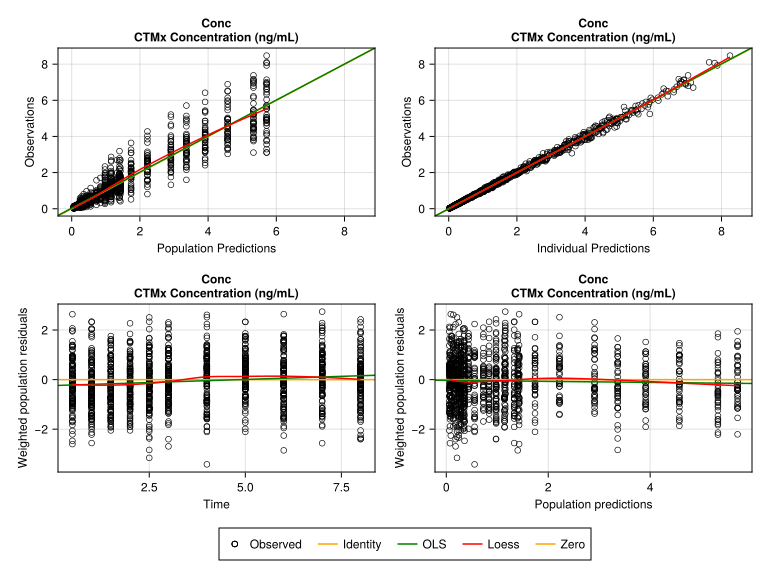
Let’s revaluate the goodness of fits and η distribution plots.
Not much change in the general gof plots
res_inspect_2cmp_unfix_ka = inspect(pkfit_2cmp_unfix_ka)[ Info: Calculating predictions. [ Info: Calculating weighted residuals. [ Info: Calculating empirical bayes. [ Info: Evaluating dose control parameters. [ Info: Evaluating individual parameters. [ Info: Done.
FittedPumasModelInspection

Likelihood approximation used for weighted residuals: FOCEgoodness_of_fit(
res_inspect_2cmp_unfix_ka;
figure = (; fontsize = 12),
legend = (; position = :bottom),
)
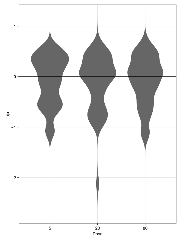
But you can see a huge improvement in the ηka, (η₃) distribution which is now centered around zero
empirical_bayes_vs_covariates(
    res_inspect_2cmp_unfix_ka;
    categorical = [:Dose],
    ebes = [:η₃],
    figure = (; size = (600, 800)),
)
Finally looking at some individual plots for the same subjects as earlier:
fig_subject_fits2 = subject_fits(
    res_inspect_2cmp_unfix_ka;
    separate = true,
    paginate = true,
    facet = (; linkyaxes = false),
    figure = (; fontsize = 18),
    axis = (; xlabel = "Time (hr)", ylabel = "CTMx Concentration (ng/mL)"),
)
fig_subject_fits2[6]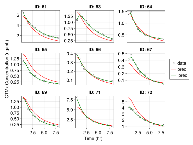
The randomly sampled individual fits don’t seem good in some individuals, but we can evaluate this via a vpc to see how to go about.
3.4 Visual Predictive Checks (VPC)
We can now perform a vpc to check. The default plots provide a 80% prediction interval and a 95% simulated CI (shaded area) around each of the quantiles
pk_vpc = vpc(pkfit_2cmp_unfix_ka, 200; observations = [:Conc], stratify_by = [:Dose])[ Info: Continuous VPC
Visual Predictive Check
  Type of VPC: Continuous VPC
  Simulated populations: 200
  Subjects in data: 120
  Stratification variable(s): [:Dose]
  Confidence level: 0.95
VPC lines: quantiles ([0.1, 0.5, 0.9])vpc_plot(
pk_2cmp,
pk_vpc;
rows = 1,
columns = 3,
figure = (; size = (1400, 1000), fontsize = 22),
axis = (;
xlabel = "Time (hr)",
ylabel = "Observed/Predicted\n CTMx Concentration (ng/mL)",
),
facet = (; combinelabels = true),
)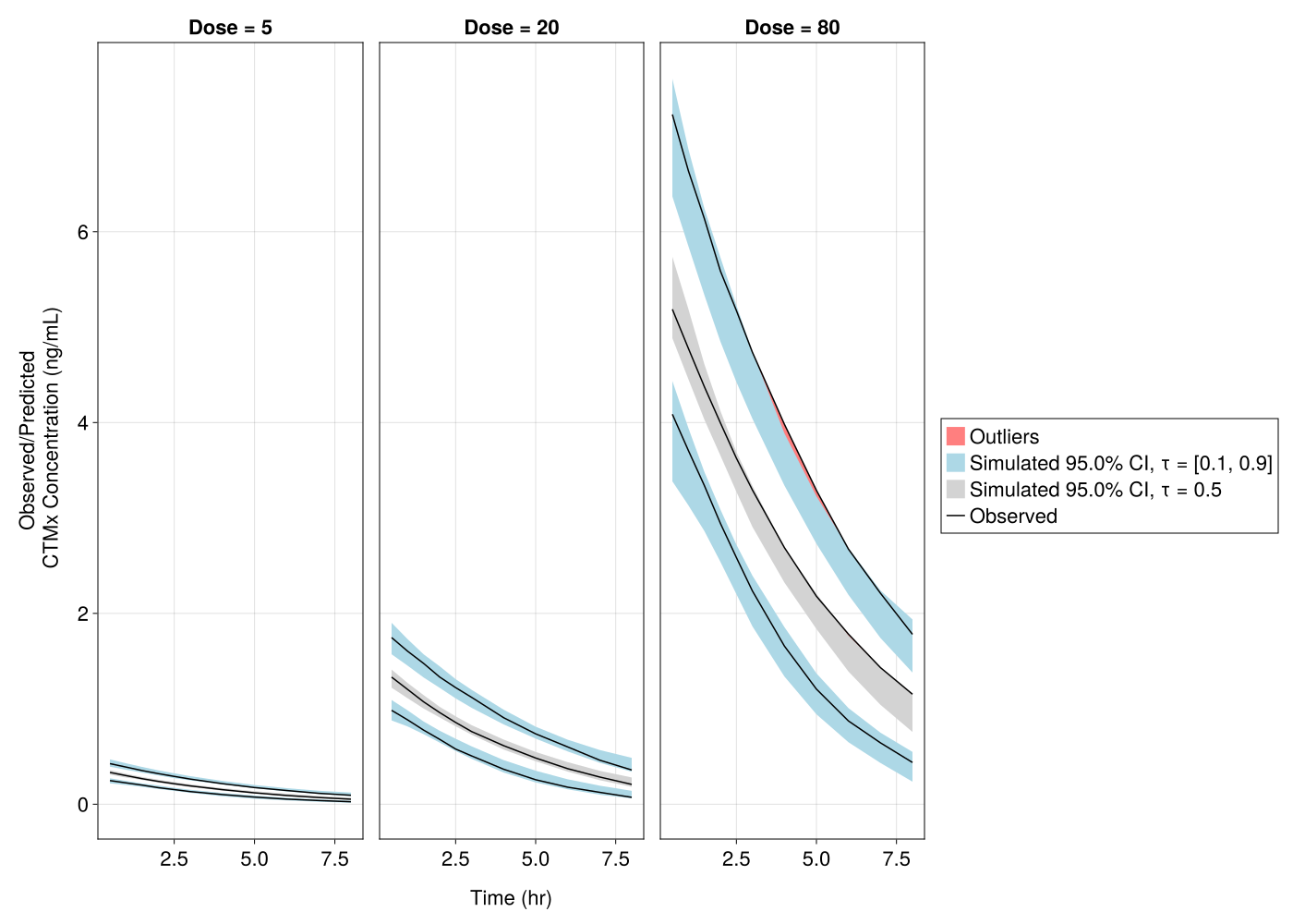
The visual predictive check suggests that the model captures the data well across all dose levels.
4 Additional Help
If you have questions regarding this tutorial, please post them on our discourse site.