Model Selection Methods - Running in a Distributed Batch Job

Batch Jobs

Please note that Batch Jobs are only available for Pumas in the Cloud, since it uses JuliaHub to run and coordinate the batch jobs.

Batch jobs are a way to easily deploy and run any piece of Julia code in a distributed manner. This means that you can run your code in parallel across multiple machines, which can be very useful for computationally intensive tasks. If you are familiar with cluster computing, batch jobs are similar to submitting a job to a cluster, but with a much simpler interface.

In order to run a batch job, you’ll need to use the JuliaHub VS Code extension. It is available by default in your Pumas environment.

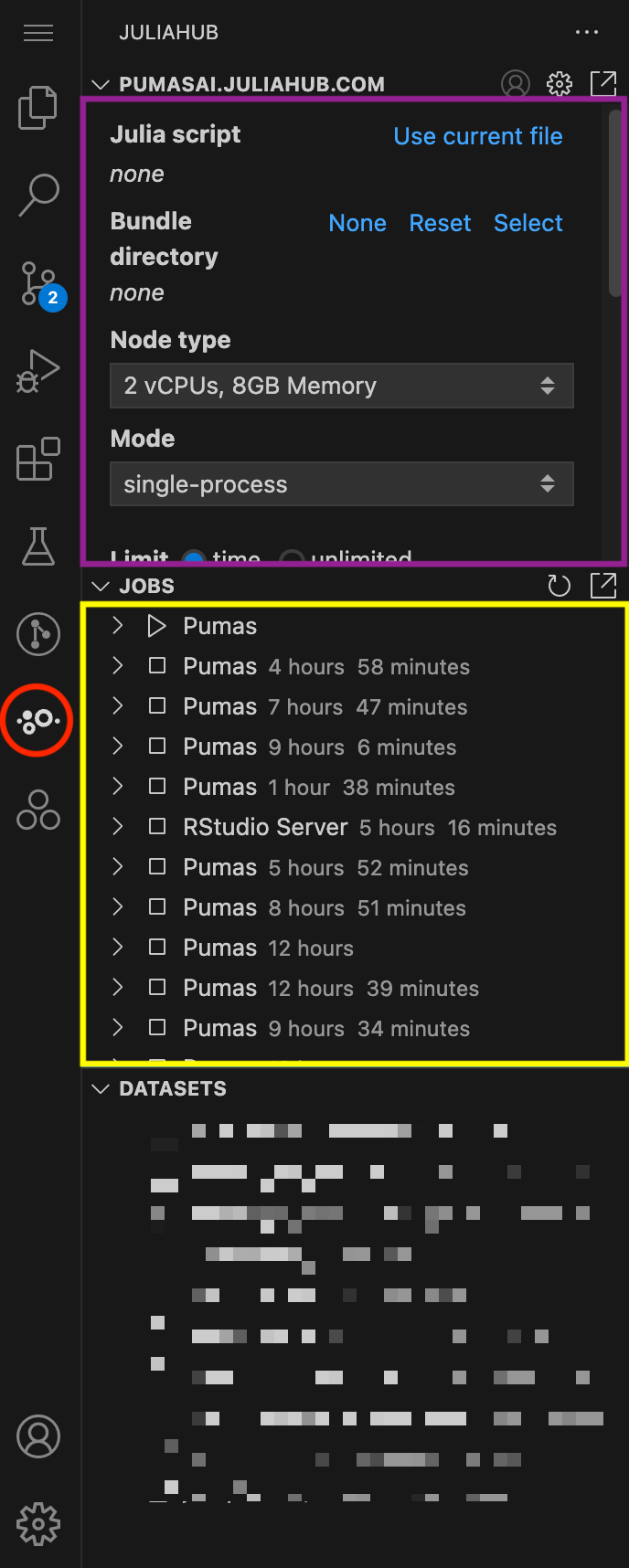
In Figure 1, we show an overview of the JuliaHub extension. It can be accessed by clicking on the JuliaHub icon in the left sidebar of VS Code (red circle). The extension provides three main subpanels:

1. Batch Jobs (in purple): This is where you can submit batch jobs.
2. Jobs Overview (in yellow): This is where you can monitor all jobs, including batch jobs and regular Apps that you have running or have run.
3. Datasets (blurred): This is where you can upload and manage datasets.

Figure 1: Julia Hub Extension Overview

Let’s focus for now on the Batch Jobs subpanel. In Figure 2 you can see it in more detail. This is where you can submit a new batch job.

Figure 2: Julia Hub Extension Batch Job Panel

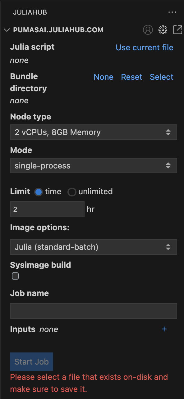
First, you need to select a script that will run in a distributed manner. This can be accomplished by filling the Julia script field with the path to the script. For convenience, you can also click on Use current file to use the currently open file in the editor.

Second, the Bundle directory will be automatic selected to the directory of the script. This is what will be sent along with the script to each individual machine that will run the batch job together. You can also select a different directory if you need to.

Bundle Directory

The bundle directory should contain all the files that the script will need to run. You can use .juliabundleignore to exclude files from the bundle directory. It functions the same way as .gitignore or .dockerignore files. Please refer to the gitignore documentation for more information.

The bundle directory can be up to 2GB in size. If you need to send more data to the machines, you should use the Datasets subpanel to upload the data. To learn more about Datasets, please check the Pumas’ Onboarding Video Tutorials

Further down, you can select the Node type. This will specify the specifications of the machines that will run the batch job.

The Mode can be either single-process or distributed. You should use distributed if you want to run the batch job in parallel across multiple machines. Once you select the distributed mode, new options will appear for you. In Figure 3 you can see the different options that you can set for the distributed mode.

Figure 3: Julia Hub Extension Batch Job Distributed Mode Options

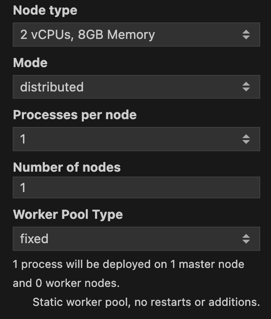
Processes per node specifies how many Julia processes will be run in each machine. In doubt you can leave it as the default value of 1 as the standard approach for a batch job is to use many nodes with just one process per node. Number of nodes specifies how many machines will be used to run the batch job. Along with Node type, Number of nodes will be the most important parameters to set. The more nodes you use, the faster the batch job will run. A caveat is that one node will be assigned as the master node, and all the others will be worker nodes. This means that the master node will not be used to run the batch job, but to orchestrate the workers. Just be mindful that the more nodes you use, the more expensive the batch job will be. So always consult with your budget before running a batch job.

Distributed Jobs and Node Type

If you are using the distributed mode, the Julia process that will run in each worker will only have access to a single thread. This means that you should select a Node type that has a lower number of vCPUs, and you should scale the number of workers instead.

Speaking of costs, it is always best practice to set a Limit for the batch job, as shown in Figure 2. By default it is set to 2 hr. Note that you do have the option to set it to unlimited, but this is not recommended.

You can also set a Worker Pool Type. You can choose between fixed and elastic. fixed will keep the number of workers constant throughout the batch job. elastic will allow the number of workers to change during the batch job.

Continuing with the options, you can set a image type in Image options. Since most of the time you will be running Pumas code, you can select the value of Pumas. Note, that we have the select box for Sysimage build. This tells JuliaHub to use a custom system image for the batch job. This should be selected only when using Pumas images.

Finally, you can set a Job name for the batch job. That will be useful to identify the batch job in the Jobs subpanel.

Once you have set all the options, you should have something like this in Figure 4.

Figure 4: Julia Hub Extension Batch Job Panel Filled

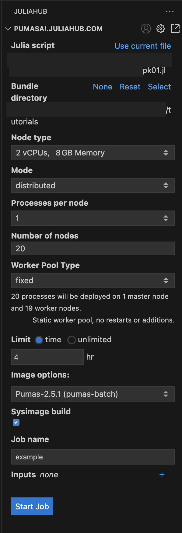
As you can see we have the pk01.jl as the Julia script, the bundle directory is the same as the script: tutorials; and we have the following options:

• Node type: 2 vCPUs, 8GB Memory
• Mode: distributed
• Processes per node: 1
• Number of nodes: 20
• Worker Pool Type: fixed
• Limit: 4 hr
• Image options: Pumas-2.5.1 (pumas-batch)
• Sysimage build: true
• Job name: example

Once you have set all the options, you can click on the Start Job button to submit the batch job. But let’s dive into some details about the script that you will run in the batch job.

1 The Script

The way you write the script will be very similar to how you would write a script to run in a single machine. However, there are three main differences that you should be aware of:

1. The use of the Distributed package and the @everywhere macro
2. EnsembleDistributed() instead of EnsembleThreads() or EnsembleSerial()
3. Save your results in a file that will be available once the batch job is finished

1.1 The use of the Distributed package and the @everywhere macro

In a batch job, you’ll have to use the Distributed package to run the code in parallel. You need to use the @everywhere macro to define functions and variables that will be available to all the workers. This is necessary because each worker will run in a different machine, and they will not have access to the same environment as the master node.

Here’s how the top of the script should look like with the Distributed package and the @everywhere macro:

using Distributed
using PharmaDatasets

@everywhere begin
    using Pumas
    using DataFramesMeta
    using PumasUtilities
    # more using statements if necessary
end

Here the master node will be using the Distributed package. And all nodes, including the master and worker nodes, will have access to Pumas, DataFramesMeta, and PumasUtilities. This is a common setup for a Pumas script.

Using @everywhere

Like all other macros in Pumas and Julia, you can employ a begin … end block to include multiple lines of code.

So, instead of writing:

@everywhere using Pumas
@everywhere using DataFramesMeta
@everywhere using PumasUtilities

You can write:

@everywhere begin
    using Pumas
    using DataFramesMeta
    using PumasUtilities
end

Since this script will not run in your local machine, i.e. not in an interactive way, it is always good practice to add some @info statements to the script. This will help you to monitor the progress of the batch job.

Here’s a toy example of a script with @info statements:

@info "Starting the batch job"

# some expensive computation
sleep(10)

@info "Finishing the batch job"

[ Info: Starting the batch job
[ Info: Finishing the batch job

@info statements

Note that you can play with timestamps and durations using the Dates package. For example, you can use Dates.now() to get the current time, and Dates.now() - start_time to get the duration of the batch job.

For more information about the Dates package, please check the Julia’s documentation.

1.2 EnsembleDistributed() instead of EnsembleThreads() or EnsembleSerial()

The second difference is that you will need to adjust all the ensemblealg options in parallel functions to use EnsembleDistributed() instead of the default EnsembleThreads() or EnsembleSerial(). This is necessary because the batch job will run in parallel across multiple machines, and you need to use EnsembleDistributed() to coordinate the parallelism across the workers.

Here’s an example of a simobs call that uses EnsembleDistributed():

sims = simobs(model, population, param; obstimes, ensemblealg = EnsembleDistributed())

And here’s an example of Bootstrap confidence interval calculation that uses EnsembleDistributed():

ci = infer(model_fit, Bootstrap(; samples = 2_000, ensemblealg = EnsembleDistributed()))

ensemblealg options

In some Pumas functions, the ensemblealg option is used to specify the parallel algorithm to use. Depending on the function, the default value of ensemblealg is EnsembleThreads() or EnsembleSerial().

For example, take a look at the help documentation for the simobs function. It uses ensemblealg = EnsembleSerial() by default. Whereas the Bootstrap function uses ensemblealg = EnsembleThreads() by default.

1.3 Save your results in a file that will be available once the batch job is finished

Finally, you should save your results in a file that will be available once the batch job is finished. This should be saved to an environment variable called RESULTS_FILE.

There are several ways to accomplish this. A good best practice is to create a temporary file and save the results there.

Here’s an example with a temporary file that has the .jls extension:

result_filename = tempname() * ".jls"

"/tmp/jl_O5SH4lgXgT.jls"

Here we are using string concatenation to add the .jls extension to the temporary file. You can use more informative file names if you want:

result_filename = tempname() * "-covariate_select_Pumas2.5.1" * ".jls"

"/tmp/jl_ghgJ2xYPwh-covariate_select_Pumas2.5.1.jls"

Temporary File

Note that you can change the extension of the temporary file to whatever you want. The most used extensions are .jls and .csv.

You will use .jls if you want to save the results in a serialized binary to use with the Serialization module. And you will use .csv if you want to save the results in a CSV file.

Serialization Compatibility

If you are using the Serialization module to save your results, note that the files generated by the Serialization module cannot be guaranteed to be compatible across different versions of Julia.

That’s why we are hardcoding the Pumas version in the file name in the example above.

To create an environment variable with the name RESULTS_FILE and the value of the result_filename, you can use the ENV dictionary that provides a dictionary interface to system environment variables where each key is a string representing an environment variable name:

ENV["RESULTS_FILE"] = result_filename

"/tmp/jl_ghgJ2xYPwh-covariate_select_Pumas2.5.1.jls"

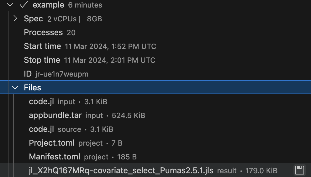
Once the batch job is finished, the file that was saved in the RESULTS_FILE environment variable will be available for download inside the Jobs subpanel of the JuliaHub extension. Here’s an example in Figure 5. We have a file named jl_X2hQ167MRq-covariate_select_Pumas2.5.1.jls that is available for download.

Figure 5: Julia Hub Extension Batch Job Results

Monitoring the Batch Job

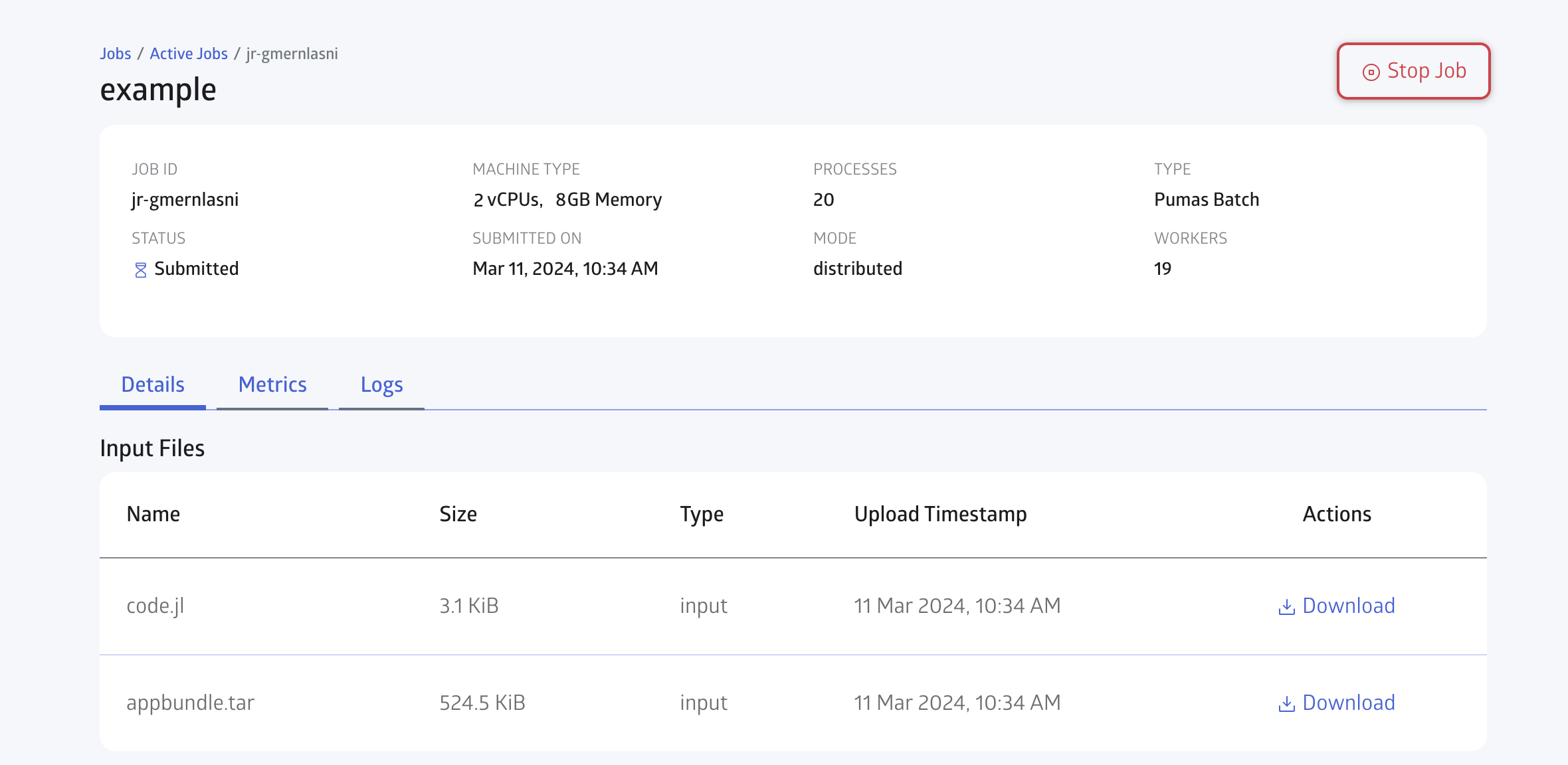
You can open the JuliaHub Jobs dashboard in your browser to monitor the progress of the batch job. In Figure 6, we show the Jobs dashboard with a batch job running.

Figure 6: Julia Hub Extension Batch Job Monitoring Dashboard

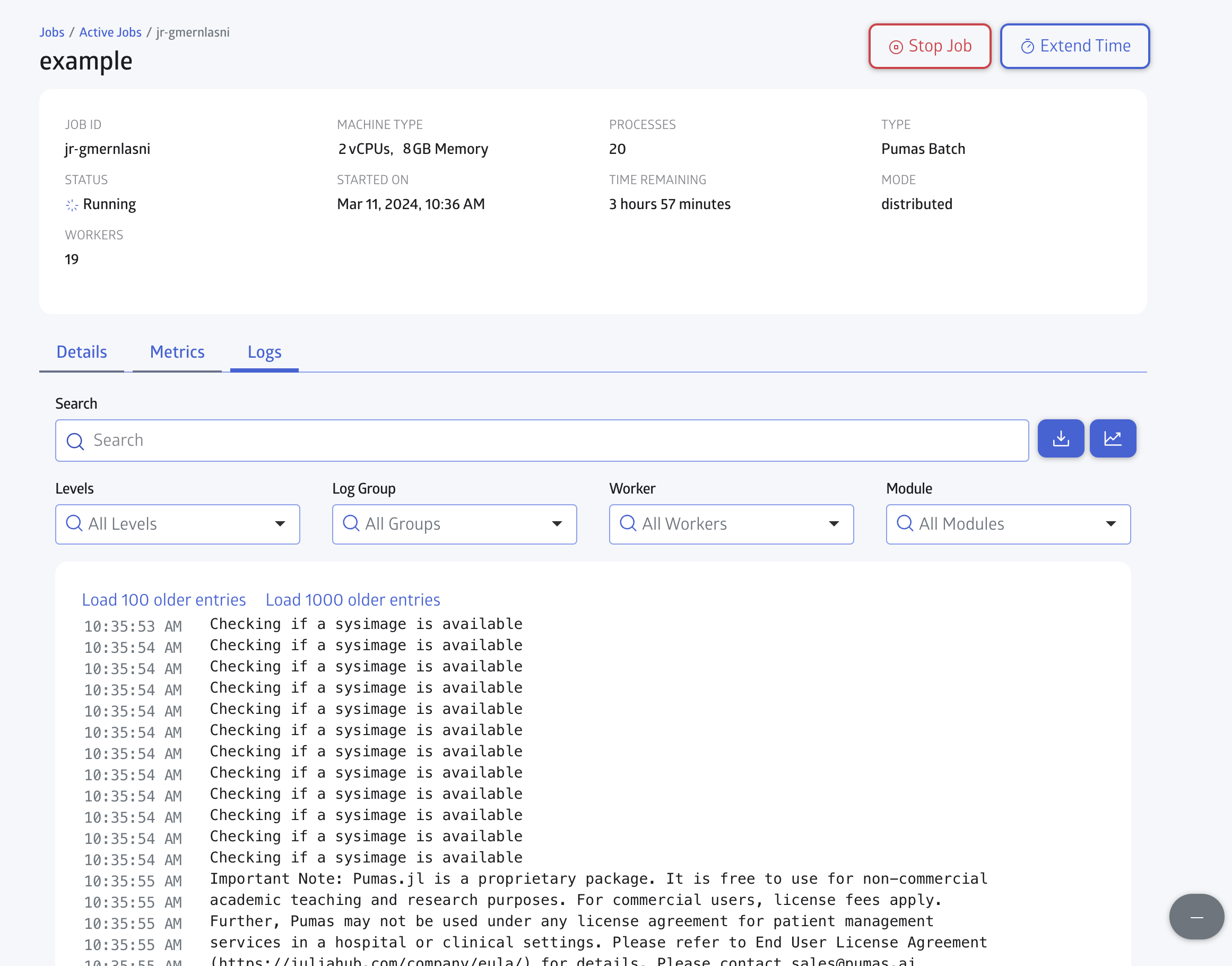
You can check for the Logs in realtime as shown in Figure 7:

Figure 7: Julia Hub Extension Batch Job Monitoring Logs

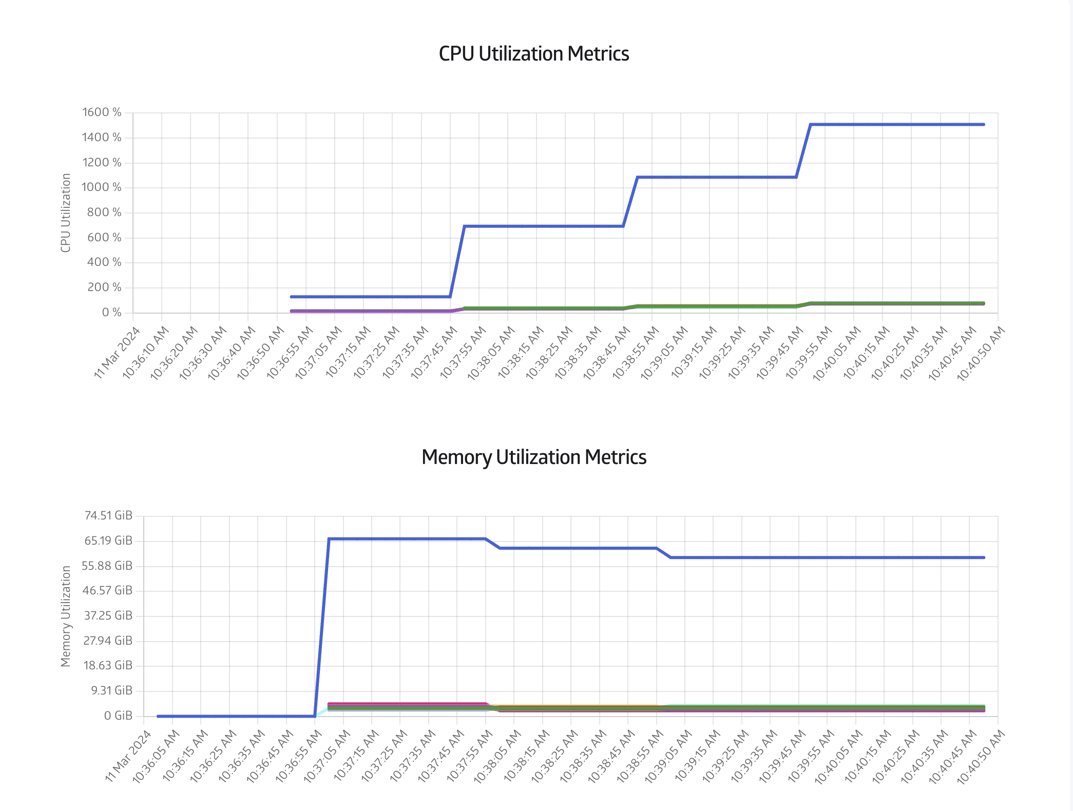
Finally you can also monitor the CPU and Memory usage in the Metrics tab, as shown in Figure 8:

Figure 8: Julia Hub Extension Batch Job Monitoring Usage

Tip

A convenient property of batch jobs is that once it has started, the instance we used to start the batch job can expire or be terminated, and batch job will still be run until completion.

This means that you don’t need to keep the current instance running to monitor the batch job. You can even close the Editor and JuliaHub altogether and the batch job will still be running.

Dry Run

It is always good practice to do a dry run of the batch job before running it for real. This will help you to check if everything is set up correctly, and if the script is running as expected.

The dry run should be done with a small dataset (maybe one or two subject(s)), and a small subset of covariates (maybe also one or two covariate(s)).

2 Example in Pumas

Let’s showcase an example that builds from the model we used in Covariate Selection Methods - Introduction.

2.1 po_sad_1 Dataset

We are going to use the po_sad_1 dataset from PharmaDatasets:

df = dataset("po_sad_1")
first(df, 5)

5×14 DataFrame

Row	id	time	dv	amt	evid	cmt	rate	age	wt	doselevel	isPM	isfed	sex	route
	Int64	Float64	Float64?	Float64?	Int64	Int64?	Float64	Int64	Int64	Int64	String3	String3	String7	String3
1	1	0.0	missing	30.0	1	1	0.0	51	74	30	no	yes	male	ev
2	1	0.25	35.7636	missing	0	missing	0.0	51	74	30	no	yes	male	ev
3	1	0.5	71.9551	missing	0	missing	0.0	51	74	30	no	yes	male	ev
4	1	0.75	97.3356	missing	0	missing	0.0	51	74	30	no	yes	male	ev
5	1	1.0	128.919	missing	0	missing	0.0	51	74	30	no	yes	male	ev

This is an oral dosing (route = "ev") NMTRAN-formatted dataset. It has 18 subjects, each with 1 dosing event (evid = 1) and 18 measurement events (evid = 0); and the following covariates:

• age: age in years (continuous)
• wt: weight in kg (continuous)
• doselevel: dosing amount, either 30, 60 or 90 milligrams (categorical)
• isPM: subject is a poor metabolizer (binary)
• isfed: subject is fed (binary)
• sex: subject sex (binary)

Let’s parse df into a Population with read_pumas:

population =
    read_pumas(df; observations = [:dv], covariates = [:wt, :isPM, :isfed], route = :route)

Population
  Subjects: 18
  Covariates: wt, isPM, isfed
  Observations: dv

2.2 Model

We’ll use the same 2-compartment oral absorption model as in Covariate Selection Methods - Forward Selection and Covariate Selection Methods - Backward Elimination:

model = @model begin
    @metadata begin
        desc = "full covariate model"
        timeu = u"hr"
    end

    @param begin
        """
        Clearance (L/hr)
        """
        tvcl ∈ RealDomain(; lower = 0)
        """
        Central Volume (L)
        """
        tvvc ∈ RealDomain(; lower = 0)
        """
        Peripheral Volume (L)
        """
        tvvp ∈ RealDomain(; lower = 0)
        """
        Distributional Clearance (L/hr)
        """
        tvq ∈ RealDomain(; lower = 0)
        """
        Fed - Absorption rate constant (h-1)
        """
        tvkafed ∈ RealDomain(; lower = 0)
        """
        Fasted - Absorption rate constant (h-1)
        """
        tvkafasted ∈ RealDomain(; lower = 0)
        """
        Power exponent on weight for Clearance
        """
        dwtcl ∈ RealDomain()
        """
        Proportional change in CL due to PM
        """
        ispmoncl ∈ RealDomain(; lower = -1, upper = 1)
        """
          - ΩCL
          - ΩVc
          - ΩKa
          - ΩVp
          - ΩQ
        """
        Ω ∈ PDiagDomain(5)
        """
        Proportional RUV (SD scale)
        """
        σₚ ∈ RealDomain(; lower = 0)
    end

    @random begin
        η ~ MvNormal(Ω)
    end

    @covariates begin
        """
        Poor Metabolizer
        """
        isPM
        """
        Fed status
        """
        isfed
        """
        Weight (kg)
        """
        wt
    end

    @pre begin
        CL = tvcl * (wt / 70)^dwtcl * (1 + ispmoncl * (isPM == "yes")) * exp(η[1])
        Vc = tvvc * (wt / 70) * exp(η[2])
        Ka = (tvkafed + (isfed == "no") * (tvkafasted)) * exp(η[3])
        Q = tvq * (wt / 70)^0.75 * exp(η[4])
        Vp = tvvp * (wt / 70) * exp(η[5])
    end

    @dynamics Depots1Central1Periph1

    @derived begin
        cp := @. 1_000 * (Central / Vc)
        """
        DrugY Concentration (ng/mL)
        """
        dv ~ @. Normal(cp, cp * σₚ)
    end
end

PumasModel
  Parameters: tvcl, tvvc, tvvp, tvq, tvkafed, tvkafasted, dwtcl, ispmoncl, Ω, σₚ
  Random effects: η
  Covariates: isPM, isfed, wt
  Dynamical system variables: Depot, Central, Peripheral
  Dynamical system type: Closed form
  Derived: dv
  Observed: dv

We won’t go into details of the model definition here, please refer to the previous tutorials in this series for a more detailed explanation. Remember to code the model such that setting a parameter value to zero completely removes the corresponding covariate effect.

In the model above, we are defining the following parameters in the @param block with respect to covariate effects:

• tvkafasted: typical value of the magnitude of the isfed covariate effect on tvka
• dwtcl: typical value of the magnitude of the wt covariate efffect on tvcl
• ispmoncl: typical value of the magnitude of the isPM covariate efffect on tvcl

These will be the parameters that we will be testing for the covariate selection.

2.3 Initial Parameters

With the model done, now we define our initial parameters:

iparams = (;
    tvkafed = 0.4,
    tvkafasted = 1.5,
    tvcl = 4.0,
    tvvc = 70.0,
    tvq = 4.0,
    tvvp = 50.0,
    dwtcl = 0.75,
    ispmoncl = -0.7,
    Ω = Diagonal(fill(0.04, 5)),
    σₚ = 0.1,
)

(tvkafed = 0.4,
 tvkafasted = 1.5,
 tvcl = 4.0,
 tvvc = 70.0,
 tvq = 4.0,
 tvvp = 50.0,
 dwtcl = 0.75,
 ispmoncl = -0.7,
 Ω = [0.04 0.0 … 0.0 0.0; 0.0 0.04 … 0.0 0.0; … ; 0.0 0.0 … 0.04 0.0; 0.0 0.0 … 0.0 0.04],
 σₚ = 0.1,)

2.4 Covariate Selection

Now, we can run the covariate selection using the covariate_select function. We’ll be using the Forward Selection (FS) method with the estimation method as FOCE(), and the default criterion to use the aic function:

covariate_select function

Under the hood, the covariate_select function uses the pmap function from the Distributed package to run the covariate selection in parallel across multiple machines.

So this is one example of a function that is already prepared to run in a distributed manner without having to change the ensemblealg options. In fact, the covariate_select function does not have an ensemblealg option.

covar_result = covariate_select(
    model,
    population,
    iparams,
    FOCE();
    control_param = (:dwtcl, :tvkafasted, :ispmoncl),
)

[ Info: fitting model with zero restrictions on: dwtcl, tvkafasted, ispmoncl
[ Info: criterion: 2714.959963420873
[ Info: fitting model with zero restrictions on: tvkafasted, ispmoncl
[ Info: criterion: 2713.252922396735
[ Info: fitting model with zero restrictions on: dwtcl, ispmoncl
[ Info: criterion: 2680.0726047957905
[ Info: fitting model with zero restrictions on: dwtcl, tvkafasted
[ Info: criterion: 2702.591259599917
[ Info: current best model has zero restrictions on dwtcl, ispmoncl
[ Info: criterion improved, continuing!
[ Info: fitting model with zero restrictions on: ispmoncl
[ Info: criterion: 2678.298097810124
[ Info: fitting model with zero restrictions on: dwtcl
[ Info: criterion: 2667.720451400392
[ Info: current best model has zero restrictions on dwtcl
[ Info: criterion improved, continuing!
[ Info: fitting model with zero restrictions on: 
[ Info: criterion: 2641.585946318844
[ Info: current best model has zero restrictions on 
[ Info: criterion improved, continuing!
┌ Info: final best model summary
│   best_criterion = 2641.585946318844
└   best_zero_restrictions = ()

Pumas.CovariateSelectionResults
Criterion:                                               aic
Method:                                              Forward

Best model:
  Unrestricted parameters:       dwtcl, tvkafasted, ispmoncl
  Zero restricted parameters:                               
  Criterion value:                                   2641.59

Fitted model summary:
7×4 DataFrame
 Row │ free_parameters                   zero_parameters                   fit ⋯
     │ Tuple…                            Tuple…                            Fit ⋯
─────┼──────────────────────────────────────────────────────────────────────────
   1 │ ()                                (:dwtcl, :tvkafasted, :ispmoncl)  Fit ⋯
   2 │ (:dwtcl,)                         (:tvkafasted, :ispmoncl)          Fit
   3 │ (:tvkafasted,)                    (:dwtcl, :ispmoncl)               Fit
   4 │ (:ispmoncl,)                      (:dwtcl, :tvkafasted)             Fit
   5 │ (:dwtcl, :tvkafasted)             (:ispmoncl,)                      Fit ⋯
   6 │ (:tvkafasted, :ispmoncl)          (:dwtcl,)                         Fit
   7 │ (:dwtcl, :tvkafasted, :ispmoncl)  ()                                Fit
                                                               2 columns omitted

Again this is the same as in the previous tutorials.

2.5 Save the results

Finally, we save the results in a file that will be available once the batch job is finished. First, we need to load the Serialization module:

using Serialization

Now we’re ready to save the results in a file:

@info "Saving the results in a file"
result_filename = tempname() * "-covariate_select_Pumas2.5.1" * ".jls"
ENV["RESULTS_FILE"] = result_filename

serialize(result_filename, covar_result)
@info "Results saved in file: $result_filename"

@info "Distributed covariate selection batch job finished"

[ Info: Saving the results in a file
[ Info: Results saved in file: /tmp/jl_avKj8JU1m1-covariate_select_Pumas2.5.1.jls
[ Info: Distributed covariate selection batch job finished

3 Conclusion

In this tutorial, we’ve learned how to run a batch job in a distributed manner using the JuliaHub extension. We’ve also learned how to write a script that will run in a distributed manner, and how to save the results in a file that will be available once the batch job is finished.

We’ve also showcased an example of a script that runs a distributed covariate selection using Pumas.

4 Full Script for Distributed Covariate Selection Batch Job

Here’s the full script for the distributed covariate selection batch job. We’ve removed the @info statements for brevity:

using Distributed
using Serialization
using PharmaDatasets

@everywhere using Pumas

df = dataset("po_sad_1")

population =
    read_pumas(df; observations = [:dv], covariates = [:wt, :isPM, :isfed], route = :route)

model = @model begin
    @metadata begin
        desc = "full covariate model"
        timeu = u"hr"
    end

    @param begin
        """
        Clearance (L/hr)
        """
        tvcl ∈ RealDomain(; lower = 0)
        """
        Central Volume (L)
        """
        tvvc ∈ RealDomain(; lower = 0)
        """
        Peripheral Volume (L)
        """
        tvvp ∈ RealDomain(; lower = 0)
        """
        Distributional Clearance (L/hr)
        """
        tvq ∈ RealDomain(; lower = 0)
        """
        Fed - Absorption rate constant (h-1)
        """
        tvkafed ∈ RealDomain(; lower = 0)
        """
        Fasted - Absorption rate constant (h-1)
        """
        tvkafasted ∈ RealDomain(; lower = 0)
        """
        Power exponent on weight for Clearance
        """
        dwtcl ∈ RealDomain()
        """
        Proportional change in CL due to PM
        """
        ispmoncl ∈ RealDomain(; lower = -1, upper = 1)
        """
          - ΩCL
          - ΩVc
          - ΩKa
          - ΩVp
          - ΩQ
        """
        Ω ∈ PDiagDomain(5)
        """
        Proportional RUV (SD scale)
        """
        σₚ ∈ RealDomain(; lower = 0)
    end

    @random begin
        η ~ MvNormal(Ω)
    end

    @covariates begin
        """
        Poor Metabolizer
        """
        isPM
        """
        Fed status
        """
        isfed
        """
        Weight (kg)
        """
        wt
    end

    @pre begin
        CL = tvcl * (wt / 70)^dwtcl * (1 + ispmoncl * (isPM == "yes")) * exp(η[1])
        Vc = tvvc * (wt / 70) * exp(η[2])
        Ka = (tvkafed + (isfed == "no") * (tvkafasted)) * exp(η[3])
        Q = tvq * (wt / 70)^0.75 * exp(η[4])
        Vp = tvvp * (wt / 70) * exp(η[5])
    end

    @dynamics Depots1Central1Periph1

    @derived begin
        cp := @. 1_000 * (Central / Vc)
        """
        DrugY Concentration (ng/mL)
        """
        dv ~ @. Normal(cp, cp * σₚ)
    end
end

iparams = (;
    tvkafed = 0.4,
    tvkafasted = 1.5,
    tvcl = 4.0,
    tvvc = 70.0,
    tvq = 4.0,
    tvvp = 50.0,
    dwtcl = 0.75,
    ispmoncl = -0.7,
    Ω = Diagonal(fill(0.04, 5)),
    σₚ = 0.1,
)

covar_result = covariate_select(
    model,
    population,
    iparams,
    FOCE();
    control_param = (:dwtcl, :tvkafasted, :ispmoncl),
)

result_filename = tempname() * "-covariate_select_Pumas2.5.1" * ".jls"
serialize(result_filename, covar_result)

ENV["RESULTS_FILE"] = result_filename