PK04 (Part 2) - One-compartment oral dosing

1 Background

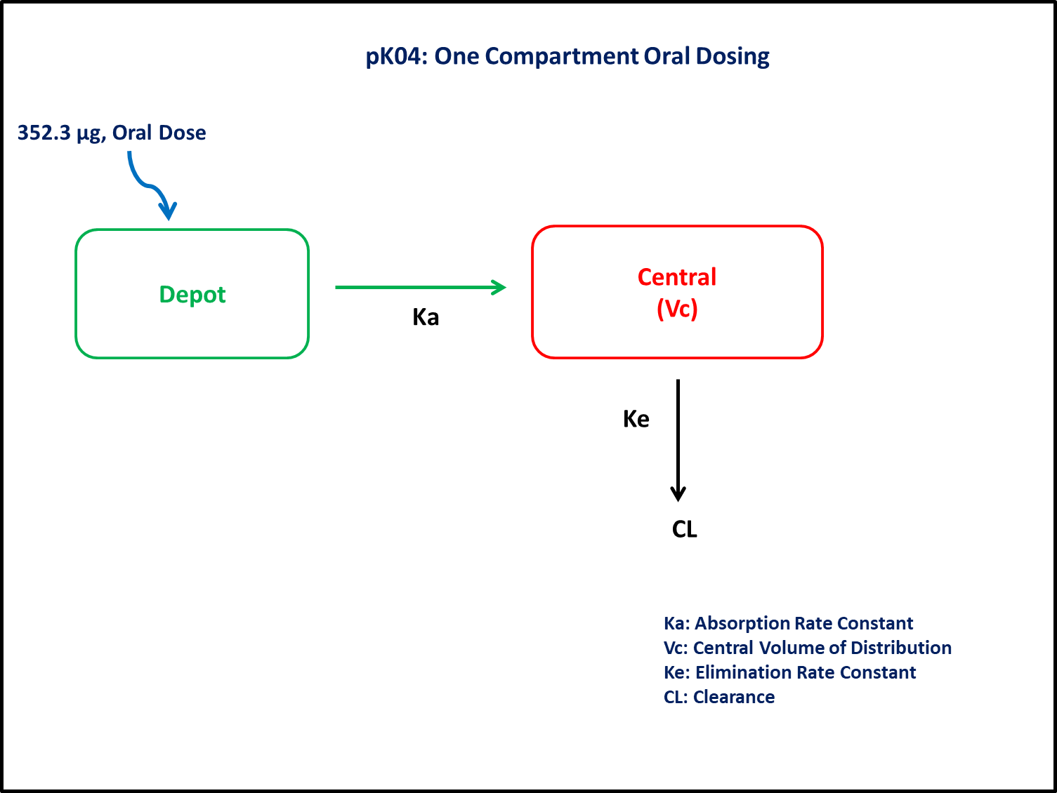
Structural model - One compartment linear elimination with first order absorption.
Route of administration - Oral, Multiple dosing
Dosage Regimen - 352.3 μg
Number of Subjects - 1

2 Learning Outcome

This exercise demonstrates simulating multiple oral dosing model kinetics from one compartment model. In exercise PK04, four models are compared.

Model 1 - One compartment model without lag-time, distinct parameters Ka and K
Model 2 - One compartment model with lag time, distinct parameters Ka and K
Model 3 - One compartment model without lag time, Ka = K = K¹
Model 4 - One compartment model with lag time, Ka = K = K¹

Models 3 and 4 are included in this tutorial, while models 1 and 2 are included in the first part

3 Objectives

To build a one-compartment model, simulate the model for a single subject given a multiple oral dosing, and subsequently perform simulation for a population.

4 Libraries

Load the necessary libraries.

using PumasUtilities
using Random
using Pumas
using CairoMakie
using AlgebraOfGraphics
using CSV
using DataFramesMeta
using Dates

5 Model definition

Note the expression of the model parameters with helpful comments. The model is expressed with differential equations. Residual variability is a proportional error model.

In this one compartment model, we administer multiple doses orally.

pk_04_3_4 = @model begin
    @metadata begin
        desc = "One Compartment Model"
        timeu = u"hr"
    end

    @param begin
        """
        Absorption & Elimination Rate Constant (1/hr)
        """
        tvk¹ ∈ RealDomain(lower = 0)
        """
        Volume of Distribution (L)
        """
        tvvc ∈ RealDomain(lower = 0)
        """
        Lag-time (hr)
        """
        tvlag ∈ RealDomain(lower = 0)
        Ω ∈ PDiagDomain(2)
        """
        Proportional RUV
        """
        σ²_prop ∈ RealDomain(lower = 0)
    end

    @random begin
        η ~ MvNormal(Ω)
    end

    @pre begin
        K¹ = tvk¹ * exp(η[1])
        Vc = tvvc * exp(η[2])
    end

    @dosecontrol begin
        lags = (Depot = tvlag,)
    end

    @dynamics begin
        Depot' = -K¹ * Depot
        Central' = K¹ * Depot - K¹ * Central
    end

    @derived begin
        """
        PK04 Concentration (μg/L)
        """
        cp = @. Central / Vc
        """
        PK04 Concentration (μg/L)
        """
        dv ~ @. Normal(cp, sqrt(cp^2 * σ²_prop))
    end
end

PumasModel
  Parameters: tvk¹, tvvc, tvlag, Ω, σ²_prop
  Random effects: η
  Covariates: 
  Dynamical system variables: Depot, Central
  Dynamical system type: Matrix exponential
  Derived: cp, dv
  Observed: cp, dv

6 Initial Estimates of Model Parameters

The model parameters for simulation are the following. Note that tv represents the typical value for parameters.

K¹ - Absorption and Elimination Rate Constant (hr⁻¹)
Vc - Volume of Central Compartment(L)
Ω - Between Subject Variability
σ - Residual error

A vector of model parameter values is defined.

param = [
    (tvk¹ = 0.14, tvvc = 56.3, tvlag = 0.0, Ω = Diagonal([0.01, 0.01]), σ²_prop = 0.015),
    (tvk¹ = 0.15, tvvc = 52.3, tvlag = 3.0, Ω = Diagonal([0.01, 0.01]), σ²_prop = 0.01),
]

7 Dosage Regimen

Dosage Regimen - 352.3 μg of oral dose once a day for 10 days.

ev1 = DosageRegimen(352.3, time = 0, ii = 24, addl = 9, cmt = 1)

1×10 DataFrame

Row	time	cmt	amt	evid	ii	addl	rate	duration	ss	route
	Float64	Int64	Float64	Int8	Float64	Int64	Float64	Float64	Int8	NCA.Route
1	0.0	1	352.3	1	24.0	9	0.0	0.0	0	NullRoute

8 Define a single-individual that receives the defined dose

pop = map(
    i -> Subject(id = i, events = ev1, observations = (cp = nothing,)),
    ["1: No Lag", "1: With Lag"],
)

Population
  Subjects: 2
  Observations: cp

9 Simulation

Simulate the plasma concentration of the drug after multiple oral dosing

Initialize the random number generator with a seed for reproducibility of the simulation.

Random.seed!(123)

Define the timepoints at which concentration values will be simulated.

sim = map(zip(pop, param)) do (subj, p)
    return simobs(pk_04_3_4, subj, p, obstimes = 0:0.1:240)
end

Simulated population (Vector{<:Subject})
  Simulated subjects: 2
  Simulated variables: cp, dv

10 Visualize Results

@chain DataFrame(sim) begin
    dropmissing(:cp)
    data(_) *
    mapping(
        :time => "Time (hours)",
        :cp => "PK04 Concentration (μg/L)",
        color = :id => "",
    ) *
    visual(Lines, linewidth = 4)
    draw(; axis = (; xticks = 0:24:240,), figure = (; fontsize = 22))
end

11 Perform a Population Simulation

We perform a population simulation with 40 participants.

This code demonstrates how to write the simulated concentrations to a comma separated file (.csv).

par4 =
    (tvk¹ = 0.15, tvvc = 52.3, tvlag = 3.0, Ω = Diagonal([0.0326, 0.0289]), σ²_prop = 0.02)

ev1 = DosageRegimen(352.3, time = 0, ii = 24, addl = 9, cmt = 1)
pop = map(i -> Subject(id = 1, events = ev1), 1:40)

Random.seed!(1234)
sim_pop = simobs(
    pk_04_3_4,
    pop,
    par4,
    obstimes = [
        1,
        2,
        3,
        4,
        5,
        6,
        7,
        8,
        10,
        12,
        14,
        24,
        216,
        216.5,
        217,
        218,
        219,
        220,
        221,
        222,
        223,
        224,
        226,
        228,
        230,
        240,
    ],
)

pkdata_04_3_4_sim = DataFrame(sim_pop)

#CSV.write("pk_04_3_4_sim.csv", pkdata_04_3_4_sim);

12 Conclusion

This tutorial showed how to build a one compartement model with and without lag time and perform a single subject and population simulation.