flowchart LR
    subgraph PK["Pharmacokinetics"]
        Dose[Drug Dose] --> Cp[Plasma<br/>Concentration Cp]
    end
    subgraph Biophase["Effect Site (Biophase)"]
        Cp -->|ke0| Ce[Effect Site<br/>Concentration Ce]
    end
    subgraph PD["Pharmacodynamics"]
        Ce --> Effect["Effect<br/>E = f(Ce)"]
    end

    style Ce fill:#fff3e0

Effect Compartment Pharmacodynamic Models
1 Learning Objectives
By the end of this tutorial, you will be able to:
- Recognize hysteresis in concentration-effect data
- Understand the effect compartment (biophase) concept
- Implement effect compartment models in Pumas
- Interpret the k_{e0} parameter and equilibration half-life
- Compare effect compartment models with direct response models
- Identify appropriate use cases for this model type
2 Introduction
When plotting drug effect against plasma concentration, we sometimes observe that the curve forms a loop rather than overlapping. This phenomenon is called hysteresis and indicates a temporal disconnect between concentration and effect.
2.1 When Direct Response Fails
Consider a patient receiving morphine for pain relief. You measure plasma concentrations and pain scores over time:
- At 1 hour: Plasma concentration is 30 ng/mL, pain score is 7
- At 3 hours: Plasma concentration is 20 ng/mL, pain score is 3
- At 6 hours: Plasma concentration is 10 ng/mL, pain score is 5
If you plot pain relief vs. concentration, the points don’t follow a single line - they form a loop. This is counter-clockwise hysteresis: the effect is lower at the same concentration during the rising phase compared to the falling phase.
NoteTypes of Hysteresis
Counter-clockwise (proteresis): Effect lags behind concentration. The drug takes time to distribute to the effect site. Modeled with an effect compartment.
Clockwise: Effect precedes or exceeds what concentration would predict. Usually indicates tolerance, receptor down-regulation, or indirect mechanisms. Typically requires different modeling approaches.
3 The Effect Compartment Concept
Sheiner et al. (1979) introduced the effect compartment (also called biophase) to explain temporal delays between plasma concentration and drug effect.
3.1 Key Principles
- The effect site is a hypothetical compartment linked to the central (plasma) compartment
- Drug equilibrates between plasma and effect site with first-order kinetics
- The effect compartment is assumed to have negligible volume (doesn’t affect PK)
- Effect is driven by the effect site concentration (C_e), not plasma concentration (C_p)
3.2 Mathematical Framework
The effect compartment is described by a first-order differential equation:
\frac{dC_e}{dt} = k_{e0} \cdot (C_p - C_e)
Where:
| Parameter | Description | Units |
|---|---|---|
| C_e | Effect site concentration | mass/volume |
| C_p | Plasma concentration | mass/volume |
| k_{e0} | First-order equilibration rate constant | 1/time |
3.3 Equilibration Half-Life
The k_{e0} parameter has a direct clinical interpretation:
t_{1/2,e0} = \frac{\ln(2)}{k_{e0}} = \frac{0.693}{k_{e0}}
This is the equilibration half-life - the time for the effect site concentration to reach 50% of the plasma concentration after a step change.
| k_{e0} (1/hr) | t_{1/2,e0} (hr) | Interpretation |
|---|---|---|
| 0.693 | 1.0 | Fast equilibration |
| 0.231 | 3.0 | Moderate equilibration |
| 0.0693 | 10.0 | Slow equilibration |
TipClinical Interpretation
A drug with t_{1/2,e0} = 30 minutes will reach ~94% equilibration between plasma and effect site within 2 hours (4 half-lives).
4 Pumas Implementation
4.1 Effect Compartment Model
effect_compartment_model = @model begin
    @metadata begin
        desc = "One-Compartment PK with Effect Compartment PD Model"
        timeu = u"hr"
    end

    @param begin
        # PK parameters
        """
        Absorption rate constant (1/hr)
        """
        pop_Ka ∈ RealDomain(; lower = 0, init = 1.0)
        """
        Clearance (L/hr)
        """
        pop_CL ∈ RealDomain(; lower = 0, init = 0.5)
        """
        Volume of distribution (L)
        """
        pop_Vc ∈ RealDomain(; lower = 0, init = 20.0)

        # PD parameters
        """
        Baseline response
        """
        pop_E0 ∈ RealDomain(; lower = 0, init = 30.0)
        """
        Maximum drug-induced effect
        """
        pop_Emax ∈ RealDomain(; lower = 0, init = 80.0)
        """
        Effect site concentration at 50% Emax
        """
        pop_EC50 ∈ RealDomain(; lower = 0, init = 1.0)
        """
        Effect site equilibration rate constant (1/hr)
        """
        pop_ke0 ∈ RealDomain(; lower = 0, init = 0.5)

        # Between-subject variability
        Ω_pk ∈ PDiagDomain(3)
        Ω_pd ∈ PDiagDomain(2)

        # Residual unexplained variability
        σ_prop_pk ∈ RealDomain(; lower = 0, init = 0.1)
        σ_add_pd ∈ RealDomain(; lower = 0, init = 3.0)
    end

    @random begin
        η_pk ~ MvNormal(Ω_pk)
        η_pd ~ MvNormal(Ω_pd)
    end

    @pre begin
        # Individual PK parameters
        CL = pop_CL * exp(η_pk[1])
        Vc = pop_Vc * exp(η_pk[2])
        Ka = pop_Ka * exp(η_pk[3])

        # Individual PD parameters
        E0 = pop_E0 * exp(η_pd[1])
        Emax = pop_Emax * exp(η_pd[2])
        EC50 = pop_EC50
        ke0 = pop_ke0
    end

    @init begin
        # Effect compartment starts at zero (no drug initially)
        Ce = 0.0
    end

    @vars begin
        # Effect site concentration for output
        Ceff = Ce
        # Plasma concentration (for plotting)
        Cp = Central / Vc
        # Predicted effect (for plotting)
        Effect = E0 + (Emax * Ce) / (EC50 + Ce)
    end

    @dynamics begin
        # PK dynamics
        Depot' = -Ka * Depot
        Central' = Ka * Depot - (CL / Vc) * Central

        # Effect compartment dynamics
        # Ce equilibrates toward Cp with rate ke0
        Ce' = ke0 * (Central / Vc - Ce)
    end

    @derived begin
        # Observations with residual error
        conc ~ @. ProportionalNormal(Cp, σ_prop_pk)
        effect ~ @. Normal(Effect, σ_add_pd)
    end
end
PumasModel
Parameters: pop_Ka, pop_CL, pop_Vc, pop_E0, pop_Emax, pop_EC50, pop_ke0, Ω_pk, Ω_pd, σ_prop_pk, σ_add_pd
Random effects: η_pk, η_pd
Covariates:
Dynamical system variables: Depot, Central, Ce
Dynamical system type: Matrix exponential
Derived: conc, effect, Ceff, Cp, Effect
Observed: conc, effect, Ceff, Cp, Effect4.2 Understanding the Model Structure
The effect compartment dynamics are key:
Ce' = ke0 * (Central / Vc - Ce)This says:
- C_e changes proportionally to the difference between C_p and C_e
- When C_p > C_e: C_e increases (drug distributing into effect site)
- When C_p < C_e: C_e decreases (drug redistributing out)
- Rate is governed by k_{e0}
The @init block sets C_e = 0 at time zero. This assumes no drug at the effect site before dosing.
The effect is calculated from C_e, not C_p:
Effect := @. E0 + (Emax * Ce) / (EC50 + Ce)This is why the effect lags behind concentration.
5 Simulation Workflow
5.1 Comparing Cp and Ce
Let’s visualize how the effect site concentration lags behind plasma concentration:
# Parameters with moderate ke0 (t1/2,e0 ≈ 1.4 hr)
params_ec = (
    pop_Ka = 1.5,
    pop_CL = 0.5,
    pop_Vc = 20.0,
    pop_E0 = 30.0,
    pop_Emax = 80.0,
    pop_EC50 = 1.0,
    pop_ke0 = 0.5,  # t1/2,e0 = 0.693/0.5 ≈ 1.4 hr
    Ω_pk = Diagonal([0.04, 0.04, 0.04]),
    Ω_pd = Diagonal([0.04, 0.04]),
    σ_prop_pk = 0.1,
    σ_add_pd = 3.0,
)

# Dosing regimen
dosing = DosageRegimen(100, time = 0, cmt = 1)

# Single subject
subject = Subject(id = 1, events = dosing)

# Simulate (without residual error for clean visualization)
sim_ec = simobs(
    effect_compartment_model,
    subject,
    params_ec,
    obstimes = 0:0.25:24,
    simulate_error = false,
)
SimulatedObservations
Simulated variables: conc, effect, Ceff, Cp, Effect
Time: 0.0:0.25:24.0# Convert simulation to DataFrame
sim_df = DataFrame(sim_ec)
dropmissing!(sim_df, [:Cp, :Ceff]) # Ensure no missing values for plotting
# Reshape data for plotting Cp and Ce together
conc_df = stack(
select(sim_df, :time, :Cp, :Ceff),
[:Cp, :Ceff];
variable_name = :concentration_type,
value_name = :concentration,
)
conc_df.concentration_type =
replace.(
string.(conc_df.concentration_type),
"Cp" => "Cp (plasma)",
"Ceff" => "Ce (effect site)",
)
# Create plot
plt =
data(conc_df) *
mapping(
:time => "Time (hr)",
:concentration => "Concentration (mg/L)",
color = :concentration_type => "Type",
) *
visual(Lines, linewidth = 2)
# Find Tmax for each
cp_max_idx = argmax(sim_df.Cp)
ce_max_idx = argmax(sim_df.Ceff)
tmax_df = DataFrame(
time = [sim_df.time[cp_max_idx], sim_df.time[ce_max_idx]],
concentration = [sim_df.Cp[cp_max_idx], sim_df.Ceff[ce_max_idx]],
concentration_type = ["Cp (plasma)", "Ce (effect site)"],
)
tmax_plt =
data(tmax_df) *
mapping(:time, :concentration, color = :concentration_type => "Type") *
visual(Scatter, markersize = 12)
draw(
plt + tmax_plt;
axis = (title = "Plasma vs Effect Site Concentration", width = 700, height = 400),
)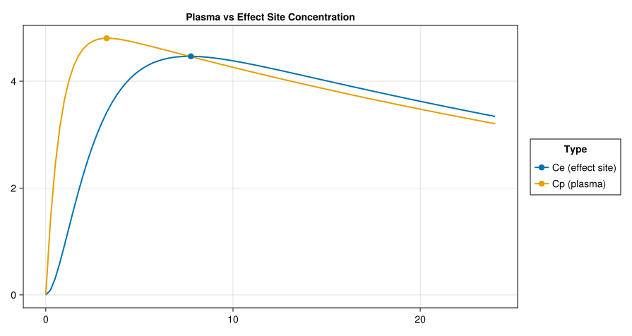
NoteKey Observation
Notice that C_e peaks later than C_p, is always lower than C_p during the absorption phase, and can exceed C_p during the elimination phase (when C_p is falling faster).
5.2 Visualizing Hysteresis
The hallmark of an effect compartment model is hysteresis in the effect-concentration plot:
# Use sim_df from previous code block (Cp and Effect are in @vars, no missing values)
hysteresis_df = select(sim_df, :Cp, :Effect)
conc = hysteresis_df.Cp
eff = hysteresis_df.Effect

# Create base hysteresis plot
plt =
    data(hysteresis_df) *
    mapping(:Cp => "Plasma Concentration (mg/L)", :Effect => "Effect") *
    visual(Lines, linewidth = 2, color = :purple)

fig = Figure(size = (600, 500))
ax = Axis(
    fig[1, 1],
    xlabel = "Plasma Concentration (mg/L)",
    ylabel = "Effect",
    title = "Effect vs Plasma Concentration (Hysteresis)",
)
draw!(ax, plt)

# Add arrows to show direction (every 4th point)
for i = 4:4:length(conc)-1
    dx = conc[i+1] - conc[i]
    dy = eff[i+1] - eff[i]
    arrows2d!(
        ax,
        [conc[i]],
        [eff[i]],
        [dx * 0.5],
        [dy * 0.5],
        color = :purple,
        shaftwidth = 1,
        minshaftlength = 0,
        tiplength = 7.5,
        tipwidth = 7.5,
    )
end

# Mark start and end
scatter!(
    ax,
    [conc[1]],
    [eff[1]],
    markersize = 15,
    color = :green,
    marker = :circle,
    label = "Start (t=0)",
)
scatter!(
    ax,
    [conc[end]],
    [eff[end]],
    markersize = 15,
    color = :red,
    marker = :star5,
    label = "End (t=24h)",
)

# Add text for loop direction
text!(ax, 2.5, 75, text = "Counter-clockwise\n(proteresis)", fontsize = 14)

axislegend(ax, position = :rb)
fig
5.3 Impact of ke0 on Delay
Let’s compare different k_{e0} values to see how they affect the delay:
ke0_values = [0.2, 0.5, 2.0]
labels = ["ke0 = 0.2 (slow)", "ke0 = 0.5 (moderate)", "ke0 = 2.0 (fast)"]

# Simulate for each ke0 value and collect results (no residual error for visualization)
ke0_results = map(zip(ke0_values, labels)) do (ke0, label)
    params_var = merge(params_ec, (; pop_ke0 = ke0))
    sim_var = simobs(
        effect_compartment_model,
        subject,
        params_var,
        obstimes = 0:0.25:24,
        simulate_error = false,
    )
    df = DataFrame(sim_var)
    df.ke0_label .= label
    df
end
ke0_df = vcat(ke0_results...)

# Time course plot
time_plt =
    data(ke0_df) *
    mapping(:time => "Time (hr)", :Effect => "Effect", color = :ke0_label => "ke0") *
    visual(Lines, linewidth = 2)

# Hysteresis plot
hyst_plt =
    data(ke0_df) *
    mapping(
        :Cp => "Plasma Concentration",
        :Effect => "Effect",
        color = :ke0_label => "ke0",
    ) *
    visual(Lines, linewidth = 2)

fig = Figure(size = (900, 400))
draw!(fig[1, 1], time_plt; axis = (title = "Effect Time Course for Different ke0",))
draw!(fig[1, 2], hyst_plt; axis = (title = "Hysteresis Loops for Different ke0",))
fig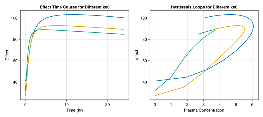
TipInterpretation
Low k_{e0} (0.2): Large hysteresis loop, effect lags significantly. High k_{e0} (2.0): Small loop, approaches direct response behavior. As k_{e0} \to \infty: No hysteresis, C_e = C_p (direct response).
6 Comparison with Direct Response
Let’s directly compare the effect compartment model with a direct response model:
# Direct response model (ke0 → infinity, effectively Cp = Ce)
direct_model = @model begin
    @metadata begin
        desc = "Direct Response for Comparison"
        timeu = u"hr"
    end

    @param begin
        pop_Ka ∈ RealDomain(; lower = 0)
        pop_CL ∈ RealDomain(; lower = 0)
        pop_Vc ∈ RealDomain(; lower = 0)
        pop_E0 ∈ RealDomain(; lower = 0)
        pop_Emax ∈ RealDomain(; lower = 0)
        pop_EC50 ∈ RealDomain(; lower = 0)
        Ω_pk ∈ PDiagDomain(3)
        Ω_pd ∈ PDiagDomain(2)
        σ_prop_pk ∈ RealDomain(; lower = 0)
        σ_add_pd ∈ RealDomain(; lower = 0)
    end

    @random begin
        η_pk ~ MvNormal(Ω_pk)
        η_pd ~ MvNormal(Ω_pd)
    end

    @pre begin
        CL = pop_CL * exp(η_pk[1])
        Vc = pop_Vc * exp(η_pk[2])
        Ka = pop_Ka * exp(η_pk[3])
        E0 = pop_E0 * exp(η_pd[1])
        Emax = pop_Emax * exp(η_pd[2])
        EC50 = pop_EC50
    end

    @dynamics begin
        Depot' = -Ka * Depot
        Central' = Ka * Depot - (CL / Vc) * Central
    end

    @vars begin
        Cp = Central / Vc
        Effect = E0 + (Emax * Cp) / (EC50 + Cp)
    end

    @derived begin
        conc ~ @. ProportionalNormal(Cp, σ_prop_pk)
        effect ~ @. Normal(Effect, σ_add_pd)
    end
end

params_direct = (
    pop_Ka = 1.5,
    pop_CL = 0.5,
    pop_Vc = 20.0,
    pop_E0 = 30.0,
    pop_Emax = 80.0,
    pop_EC50 = 1.0,
    Ω_pk = Diagonal([0.04, 0.04, 0.04]),
    Ω_pd = Diagonal([0.04, 0.04]),
    σ_prop_pk = 0.1,
    σ_add_pd = 3.0,
)

sim_direct = simobs(
    direct_model,
    subject,
    params_direct,
    obstimes = 0:0.25:24,
    simulate_error = false,
)
SimulatedObservations
Simulated variables: conc, effect, Cp, Effect
Time: 0.0:0.25:24.0# Convert both simulations to DataFrames
direct_df = DataFrame(sim_direct)
direct_df.model .= "Direct Response"
ec_df = DataFrame(sim_ec)
ec_df.model .= "Effect Compartment"
# Combine for comparison (using vars: Cp and Effect)
comparison_df = vcat(
select(direct_df, :time, :Cp, :Effect, :model),
select(ec_df, :time, :Cp, :Effect, :model),
)
# Time course plot
time_plt =
data(comparison_df) *
mapping(:time => "Time (hr)", :Effect => "Effect", color = :model => "Model") *
visual(Lines, linewidth = 2)
# Concentration-effect plot
ce_plt =
data(comparison_df) *
mapping(:Cp => "Plasma Concentration", :Effect => "Effect", color = :model => "Model") *
visual(Lines, linewidth = 2)
fig = Figure(size = (900, 400))
draw!(fig[1, 1], time_plt; axis = (title = "Effect Time Course",))
draw!(fig[1, 2], ce_plt; axis = (title = "Concentration-Effect Relationship",))
fig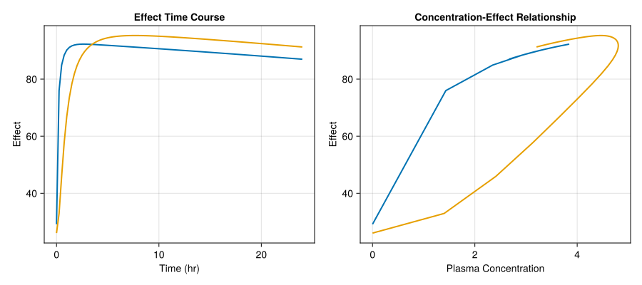
7 Population Simulation
# Create population
population = map(1:20) do i
    Subject(id = i, events = dosing)
end

# Simulate
Random.seed!(123)
sim_pop = simobs(effect_compartment_model, population, params_ec, obstimes = 0:0.5:24)
Simulated population (Vector{<:Subject})
Simulated subjects: 20
Simulated variables: conc, effect, Ceff, Cp, Effect# Convert population simulation to DataFrame
pop_df = DataFrame(sim_pop)
# Time course plot (using vars: Cp, Effect - always available for each time point)
time_pop_plt =
data(pop_df) *
mapping(:time => "Time (hr)", :Effect => "Effect", group = :id) *
visual(Lines, linewidth = 1, alpha = 0.5, color = :coral)
# Hysteresis plot
hyst_pop_plt =
data(pop_df) *
mapping(:Cp => "Plasma Concentration", :Effect => "Effect", group = :id) *
visual(Lines, linewidth = 1, alpha = 0.5, color = :coral)
fig = Figure(size = (900, 400))
draw!(fig[1, 1], time_pop_plt; axis = (title = "Population Effect Profiles",))
draw!(fig[1, 2], hyst_pop_plt; axis = (title = "Population Hysteresis",))
fig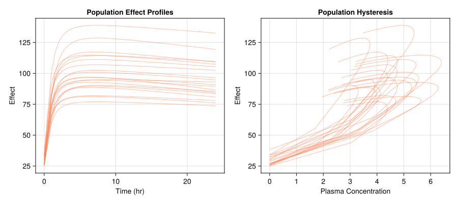
8 Fitting Workflow
8.1 Generate Synthetic Data
Random.seed!(456)
sim_data = simobs(
    effect_compartment_model,
    population,
    params_ec,
    obstimes = [0.5, 1, 2, 4, 6, 8, 12, 24],
)
df_sim = DataFrame(sim_data)
8.2 Fit the Model
fit_pop = read_pumas(
    df_sim;
    id = :id,
    time = :time,
    amt = :amt,
    evid = :evid,
    cmt = :cmt,
    observations = [:conc, :effect],
)

init_params = (
    pop_Ka = 1.2,
    pop_CL = 0.4,
    pop_Vc = 25.0,
    pop_E0 = 25.0,
    pop_Emax = 70.0,
    pop_EC50 = 0.8,
    pop_ke0 = 0.4,
    Ω_pk = Diagonal([0.02, 0.02, 0.02]),
    Ω_pd = Diagonal([0.02, 0.02]),
    σ_prop_pk = 0.15,
    σ_add_pd = 5.0,
)

fit_result = fit(effect_compartment_model, fit_pop, init_params, FOCE())
[ Info: Checking the initial parameter values. [ Info: The initial negative log likelihood and its gradient are finite. Check passed. Iter Function value Gradient norm 0 6.873912e+02 1.812684e+02 * time: 0.048448801040649414 1 6.245205e+02 6.239977e+01 * time: 4.0942299365997314 2 6.087162e+02 9.265906e+01 * time: 4.359418869018555 3 5.988677e+02 3.940733e+01 * time: 6.044734954833984 4 5.942967e+02 1.655980e+01 * time: 6.330320835113525 5 5.938042e+02 8.486321e+00 * time: 6.597376823425293 6 5.931968e+02 9.198198e+00 * time: 6.849121809005737 7 5.924225e+02 5.887526e+00 * time: 7.100631952285767 8 5.915151e+02 7.302707e+00 * time: 7.354637861251831 9 5.909802e+02 5.186712e+00 * time: 7.611262798309326 10 5.904100e+02 4.546817e+00 * time: 7.873257875442505 11 5.902566e+02 2.480408e+00 * time: 8.16219186782837 12 5.901009e+02 2.743252e+00 * time: 8.48751187324524 13 5.899501e+02 3.439750e+00 * time: 8.73558783531189 14 5.897909e+02 3.064519e+00 * time: 8.982778787612915 15 5.897048e+02 1.407096e+00 * time: 9.231827974319458 16 5.896350e+02 1.909421e+00 * time: 9.473780870437622 17 5.895451e+02 2.232333e+00 * time: 9.746332883834839 18 5.894034e+02 3.548018e+00 * time: 9.987822771072388 19 5.892658e+02 3.422145e+00 * time: 10.238601922988892 20 5.891965e+02 2.075156e+00 * time: 10.483380794525146 21 5.891788e+02 6.018433e-01 * time: 10.72635293006897 22 5.891770e+02 2.638434e-01 * time: 10.993876934051514 23 5.891763e+02 2.633735e-01 * time: 11.282909870147705 24 5.891742e+02 5.199753e-01 * time: 11.53361177444458 25 5.891703e+02 9.215953e-01 * time: 11.789265871047974 26 5.891625e+02 1.288241e+00 * time: 12.078645944595337 27 5.891524e+02 1.200225e+00 * time: 12.325301885604858 28 5.891452e+02 5.787931e-01 * time: 12.578561782836914 29 5.891434e+02 2.014071e-01 * time: 12.834218978881836 30 5.891427e+02 1.981958e-01 * time: 13.076526880264282 31 5.891417e+02 3.386368e-01 * time: 13.335749864578247 32 5.891403e+02 4.482474e-01 * time: 13.60122299194336 33 5.891389e+02 3.570436e-01 * time: 13.847304821014404 34 5.891383e+02 1.343985e-01 * time: 14.110402822494507 35 5.891382e+02 2.035602e-02 * time: 14.36039686203003 36 5.891382e+02 8.697655e-03 * time: 14.625741004943848 37 5.891382e+02 8.473242e-03 * time: 14.874677896499634 38 5.891382e+02 7.941083e-03 * time: 15.135471820831299 39 5.891382e+02 6.646330e-03 * time: 15.388293981552124 40 5.891382e+02 9.325912e-03 * time: 15.65721583366394 41 5.891382e+02 8.668836e-03 * time: 15.90943193435669 42 5.891382e+02 8.665922e-03 * time: 16.192752838134766 43 5.891382e+02 8.665453e-03 * time: 16.4998939037323 44 5.891382e+02 8.665453e-03 * time: 16.8603618144989 45 5.891382e+02 8.665453e-03 * time: 17.27327799797058 46 5.891382e+02 8.665453e-03 * time: 17.67107582092285 47 5.891382e+02 8.663914e-03 * time: 18.007847785949707 48 5.891382e+02 8.663914e-03 * time: 18.337499856948853 49 5.891382e+02 8.663914e-03 * time: 18.6766037940979
FittedPumasModel

Dynamical system type:          Matrix exponential

Number of subjects:                             20

Observation records:         Active        Missing
    conc:                       160              0
    effect:                     160              0
    Total:                      320              0

Number of parameters:      Constant      Optimized
                                  0             14

Likelihood approximation:                     FOCE
Likelihood optimizer:                         BFGS

Termination Reason:              NoObjectiveChange
Log-likelihood value:                   -589.13818

----------------------
            Estimate
----------------------
pop_Ka       1.4971
pop_CL       0.49317
pop_Vc      20.194
pop_E0      25.881
pop_Emax    85.034
pop_EC50     0.89644
pop_ke0      0.50306
Ω_pk₁,₁      0.055835
Ω_pk₂,₂      0.036068
Ω_pk₃,₃      0.028255
Ω_pd₁,₁      0.011628
Ω_pd₂,₂      0.037389
σ_prop_pk    0.10147
σ_add_pd     3.2311
----------------------
# Estimated parameters
coef(fit_result)(pop_Ka = 1.4970517674541763, pop_CL = 0.49316774712417677, pop_Vc = 20.19353318566788, pop_E0 = 25.881425881173815, pop_Emax = 85.03447624567004, pop_EC50 = 0.8964412651632103, pop_ke0 = 0.5030632112008884, Ω_pk = [0.055835142210560455 0.0 0.0; 0.0 0.03606823822650806 0.0; 0.0 0.0 0.028254512458659935], Ω_pd = [0.011628457317986793 0.0; 0.0 0.037388603847163436], σ_prop_pk = 0.10147054587188924, σ_add_pd = 3.2311064968684025)9 Model Diagnostics
insp = inspect(fit_result)[ Info: Calculating predictions. [ Info: Calculating weighted residuals. [ Info: Calculating empirical bayes. [ Info: Evaluating dose control parameters. [ Info: Evaluating individual parameters. [ Info: Done.
FittedPumasModelInspection

Likelihood approximation used for weighted residuals: FOCEgoodness_of_fit(insp; observations = [:effect])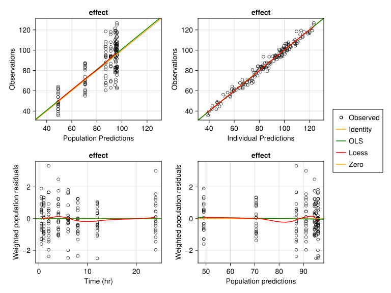
10 Clinical Examples
- Drug: Morphine (analgesic)
- Site of action: Central nervous system
- t_{1/2,e0}: ~1.5-2 hours
- Clinical implication: Pain relief lags behind plasma levels; titration requires patience
- Reference: Lotsch et al. (2006)
- Drug: Digoxin (cardiac glycoside)
- Site of action: Cardiac muscle
- t_{1/2,e0}: ~8 hours
- Clinical implication: Slow equilibration means toxicity may appear delayed
- Reference: Jelliffe (2014)
- Drug: Warfarin (anticoagulant)
- Site of action: Liver (clotting factor synthesis)
- t_{1/2,e0}: ~6-8 hours for initial effects
- Note: Full anticoagulant effect involves indirect response (clotting factor turnover)
- Reference: Hamberg et al. (2007)
11 Summary
In this tutorial, we covered:
- Hysteresis: Counter-clockwise loops in effect-concentration plots indicate effect site distribution delay
- Effect compartment: A hypothetical compartment linked to plasma that explains the delay
- k_{e0} parameter: The equilibration rate constant; t_{1/2,e0} = 0.693/k_{e0}
- Pumas implementation: Using the
@dynamicsblock for C_e dynamics - Comparison: Effect compartment → direct response as k_{e0} increases
11.1 When to Use Effect Compartment Models
- Counter-clockwise hysteresis is observed
- Peak effect occurs after peak concentration
- Drug distributes slowly to site of action
- CNS-acting drugs with blood-brain barrier
11.2 Next Steps
If your data shows:
- Effect persists long after drug clears: Consider Indirect Response Models
- Irreversible drug-target interaction: Consider K-PD Models
- Model selection challenges: See Model Selection Tutorial
References
Hamberg, A. K., M. L. Dahl, T. M. Barber, and M. Wadelius. 2007. “A PK-PD Model for Predicting the Impact of Age, CYP2C9, and VKORC1 Genotype on Individualization of Warfarin Therapy.” Clinical Pharmacology & Therapeutics 81 (4): 529–38.
Jelliffe, R. W. 2014. “Some Comments and Suggestions Concerning Population Pharmacokinetic Modeling, Especially of Digoxin, and Its Relation to Clinical Therapy.” Therapeutic Drug Monitoring 36 (5): 567–83.
Lotsch, J., C. Skarke, H. Schmidt, J. Liefhold, and G. Geisslinger. 2006. “Pharmacokinetic Modeling to Predict Morphine and Morphine-6-Glucuronide Plasma Concentrations in Healthy Young Volunteers.” Clinical Pharmacology & Therapeutics 79 (3): 278–88.
Sheiner, L. B., D. R. Stanski, S. Vozeh, R. D. Miller, and J. Ham. 1979. “Simultaneous Modeling of Pharmacokinetics and Pharmacodynamics: Application to d-Tubocurarine.” Clinical Pharmacology & Therapeutics 25 (3): 358–71.